High-level Petri Nets provide a graphical and mathematical tool for system description and analysis that can be applied effectively to issues of parallel and asynchronous workflow [1]. Vigorous research and development on Petri Nets in recent years has led to a widening of their field of application. Petri Nets have become the preferred modeling tool for net systems that have a variety of abstraction levels [2]. They have been used widely in the areas of discrete event systems analysis, flexible manufacturing systems (FMS), automatic control, computer network performance analysis and protocol verification, parallel program design and analysis, knowledge inference, artificial neural networks, and decision models [3].
One of the main purposes of using Petri Nets to model an actual system is to analyze the properties and functions of the actual system with the assistance of a system model. We research Petri Nets for the purpose of applying them to areas of artificial intelligence, such as knowledge expression and the establishment of formalized reasoning models, expressing relationships among various activities, reasoning logically based on modeling through a known initial state and initial conditions, calculating the credibility of each inference result through fuzzy inference reasoning, and determining reasonable inference results. In order to achieve this purpose, we first study the reachability of a Petri Net.
In research on Petri Nets, reachability is probably the most basic dynamic property and the decidability of the reachability problem is probably the most important open problem in the mathematical theory of Petri Nets and related formalisms. In a sense, research on reachability is the foundation for research on other dynamic properties of Petri Nets, because many other problems can be described using reachability. The reachability problem for Petri Nets is to decide, given a Petri Net
While reachability seems to be a good tool for finding erroneous states, the constructed graph usually has far too many states to calculate for practical problems. To alleviate this drawback, linear temporal logical (LTI) is customarily used in conjunction with the tableau method to prove that such states cannot be reached. LTL uses the semi-decision technique to find if a state can be reached, by finding a set of necessary conditions for the state to be reached and then proving that those conditions cannot be satisfied.
Thus, if the decision problem of reachability can be solved, then other dynamic properties such as activity are expected to be solved. Unfortunately, it is not easy to find a general algorithm that can determine the reachability of any Petri Net, especially an unbounded Petri Nets. Since the reachability decision problem has at least exponential space complexity and no effective algorithm is found by now, so if we can find and prove some Petri Net subclasses that can use the satisfiability of the state equation to decide the reachability, it is also an important and indispensable work.
It has been proved that, for the live
The rest of this paper is organized as follows. Section 2 gives a short review and comparison of related studies and then presents the contributions of our paper. Section 3 describes the basic notations and definitions of Petri Nets. Section 4 first shows two examples to illustrate why using state equations cannot decide the reachability of any kind of Petri Net, then proposed a subclass of Petri Net, that can use the satisfiability of state equation to decide the reachability, and then proved the validity. Section 5 introduces parts of existing reachability decision methods. Finally we draw conclusions and suggest future studies.
Our research relates to a number of areas, especially Petri Netbased formalisms, dynamic behavior, and synchronized concurrent systems research. Since for some subclasses of Petri Net, the state equation has non-negative integer solution is not only the necessary condition but also the sufficient condition of
Liu and Chen [6] have found a subnet of Petri Net: ∑ = (
Despite these previous researches, some other researchers devote themselves to use Petri Net as a tool for context inference, modeling and analyzing of discrete event and so on. Lee et al. [10] propose a context inference model which is based on the socalled fuzzy colored timed Petri Net. The model represents and handles the sequential occurrence of some events along with involving timing constraints, deals with the multiple entities using the colored Petri Net model, and employs the concept of fuzzy tokens to manage the fuzzy concepts [10]. Mo et al. [11] proposed a fuzzy transition timed Petri Net with fuzzy theory to determine the optimal transition time. Kim et al. [12] models traffic system with fuzzy discrete event system’s character in fuzzy transition timed Petri Net, and based on it to design a traffic signal controller.
Based on the abovementioned studies, in this paper, we put forward a subnet of a Petri Net-a live single branch Petri Net whose reachability is equivalent to the satisfiability of the state equation.
3. Basic Notations and Definitions of Petri Net
3.1 Features and Definition of Petri Net
Petri Net has many good features that can be used to analyze and describe the system. It can simulate the system from the perspective control and management, accurately describe the dependency and dependency relationship of the event of in the system, describe the system structure and behavior with unified language and describe the synchronized concurrent systems, provide a new way to solve the different kinds of problems, refer to the literature [13].
Petri Net is a model used to describe distributed systems. It can not only describe the structure of the system, but also simulate the operation of the system. The part that describes the system structure is referred to as a network. In form, a net is a directed bipartite graph without isolated nodes.
A triple
1)
2)
3)
4)
Where:
dom(F) = {x ∈ S ∪ T│∃y ∈ S ∪ T : (x, y) ∈ F}
cod(F) = {x ∈ S ∪ T│∃y ∈ S ∪ T : (y, x) ∈ F}
Suppose
?x = {y│y ∈ S ∪ T ∧ (y, x) ∈ F}
x? = {y│y ∈ S ∪ T ∧ (x, y) ∈ F}
Here we name ?
An extension of a place is the subset of transition set
Suppose
When we use a Petri Net to simulate an actual system, the net ∑ = (
Based on this, we can define the net system ∑ as follows: here
1)
2) If
For the bounded Petri Net, since its reachability marking set
Suppose ∑ = (
4. The Subclass of Petri Net with Reachability Equivalent to State Equation Satisfiability
4.1 The Limitations of Using State Equations to Decide Reachability for Any Kinds of Petri Net
For a general Petri Net, ∑ = (
In the following, we’ll use two examples to show why we cannot use the state equation to decide the reachability for any kinds of Petri Nets.
First, considering the matrix method for analyzing Petri Nets, a matrix A cannot reflect the structure of a Petri Net accurately, because if the transition section uses one position to input and output simultaneously, there will be a self-loop, i.e., the same position of A+ and A? will occur at the same number, which will be mutually offset by A? - A+.
Second, there will be missing sequence information in the triggered vector.
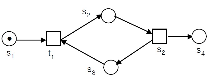
For example, suppose we want to confirm whether the identification (0, 0, 0, 0, 1) can be reached from (1, 0, 0, 0, 0) in Figure 1. If we use the state equation to decide reachability, we get Equation (1):
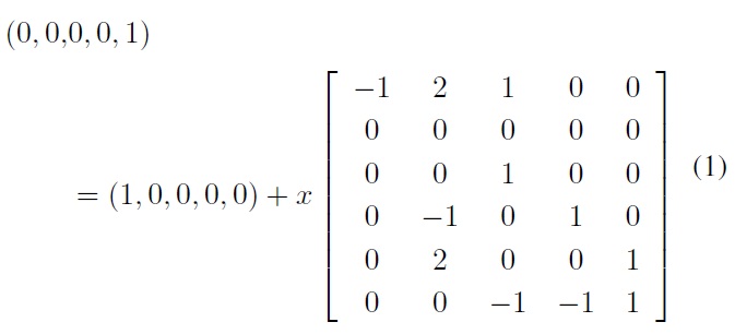
(For the matrix, the column indicate the place
Obviously, the solution of this equation is not unique. From this general form, we can know only the relationships among the numbers of the initiation of the transition node, but cannot confirm the sequence of the initiation.
Third, the solution calculated using the state equation might be a false solution.
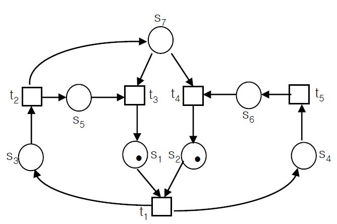
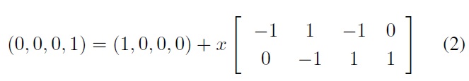
For example, suppose we want to confirm whether the identification (0, 0, 0, 1) can be reached from (1, 0, 0, 0) in Figure 2. If we use state equation to decide reachability, we can get Equation (2):
This equation has a solution of (1, 1). The equation corresponds to the two initiating sequences
However, there exits some special Petri Net, the reachability problem is easily to be decided, so it has great significant to find such Petri Net subclass. In the following, we will define
a Petri Net subclass and prove that, for this kind of Petri Net subclass, the reachability is also equivalent to the satisfiability of the state equation.
4.2 The Proposed Petri Net Subclass and Demonstration
For a Petri Net∑ = (
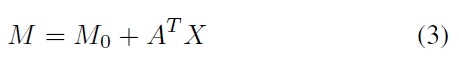
here
However, for some subclass of Petri Net, Equation (3) is the sufficient and necessary condition of
Suppose ∑ = (
Obviously the live single branch Petri Net includes the live weighted
Xu and Wu [8] have proved that for the live weighted
Since it is depicted in extensive literature that the equation
Before we prove this, we first prove two propositions.
Proposition 1:
Suppose ∑ = (
Proof:
(1) The necessity of this theorem follows obviously from the basic properties of Petri Nets.
(2) Now we prove the sufficiency
Suppose
Since
M3[ti4 > M4; ... ;MK?1[tiK > MK = Md.
Finally we can conclude that identifier
This proves the sufficiency, and thus also proposition 1.
Proposition 2:
Suppose ∑=(
Proof: We use reductio ad absurdum.
Suppose an
Algorithm:
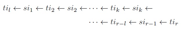
Step 0: ① Randomly select a t∈TX, labeled as til;
② S1 = {s│s ∈ ?ti1, and M0(s) < W(s, ti1) //W is the weighted function of ∑, because the //M0[til> is false, so S1≠0.
③ Counting variable j:=1;
Step l: ①Tj+1 = {t│t ∈ ?Sj, and t ∈ TX
② If Tj+1 ≠= ? then
{
Randomly select a t∈Tj+1, labeled as tij+1, and label sij as the place S of ?tij∩ t?ij+1 (here, if there are many places in ?tij ∩ t?ij+1, then select one of them randomly);
}
Else // Tj+1=?
Jump to Step 2.
③ If tij+1 = tk and 1 ≤ k ≥ j then Jump to Step 2. Else j:=j+l, Jump to Step l.
Step 2: End.
It is easy to see that since the elements in T are finite, the algorithm can be terminated. We can finally get the sequence:
We discuss the sequence
(1) Case 1:
When
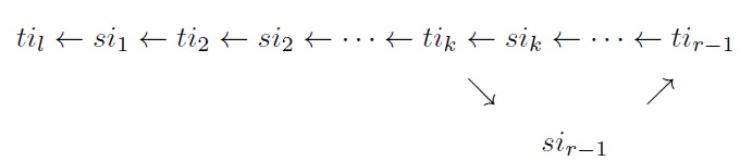
Analyze the loop
(2) Case 2:
When
(where
Since
Thus proposition 2 is proved.
Proposition 3:
Based on the above conclusions (conclusions 1 and 2) we will prove, for any live single-branch Petri Net ∑ = (
Proof:
The necessity of this theorem follows obviously from the basic properties of Petri Nets.
Now let us prove the sufficiency:
Since the ∑ = (
Then according to proposition 1, since the ∑ = (
As a result, we can draw the conclusion that: Suppose ∑ = (
Petri Nets are a tool for system description and analysis. Reachability is one of the most basic properties in Petri Net research. We research Petri Nets for the purpose of applying them to areas of artificial intelligence, such as knowledge expression and the establishment of formalized reasoning models, expressing relationships among various activities, reasoning logically based on modeling through a known initial state and initial conditions, calculating the credibility of each inference result through fuzzy inference reasoning, and determining reasonable inference results. In order to achieve this purpose, the first task is to research the reachability of Petri Nets. In a sense, reachability is the foundation of the study of other dynamic properties of Petri Nets. Many problems on Petri Nets can be described by it, so the reachability decision problem is therefore one of the most important topics in Petri Net theory.
Methods that can be used to analyze the reachability of a Petri Net include the reachable marking graph and coverability tree, the correlation matrix and state equation, and Petri Net language. Each method has its advantages and disadvantages. Sometimes we can combine them, so as to analyze the dynamic properties of a Petri Net.
Although, using state equation cannot decide the reachability for all kinds of Petri Net, bur since this method is very easy to be grasped and is convenient to be used without the judgment of the existence of legitimate sequence, so if we can prove that for some kinds of Petri Net subclasses, the state equation satisfiability is not only a necessary condition but also a sufficient condition, then it is also an important and indispensable work.
The previous researches have proved that some subclass of Petri Net, such as transition-single-input-circuit Petri Nets, minimum-transition-single-input-trap-circuit Petri Nets, minimumsiphon- circuit Petri Nets, and live weighted
Based on these previous researches, we found a subclass that includes the live weighted
However, our proposed method is suitable only for determining the reachability of a subclass of a Petri Net, so in the future, the key issue in our further study will be to determine how to combine our proposed method in this paper with an improved coverability tree proposed in reference [15] to decide reachability for a general Petri Net.
No potential conflict of interest relevant to this article was reported.