


We pose pattern classification as a density estimation problem where we consider mixtures of generative models under partially labeled data setups. Unlike traditional approaches that estimate density everywhere in data space, we focus on the density along the decision boundary that can yield more discriminative models with superior classification performance. We extend our earlier work on the recursive estimation method for discriminative mixture models to semi-supervised learning setups where some of the data points lack class labels. Our model exploits the mixture structure in the functional gradient framework: it searches for the base mixture component model in a greedy fashion, maximizing the conditional class likelihoods for the labeled data and at the same time minimizing the uncertainty of class label prediction for unlabeled data points. The objective can be effectively imposed as individual mixture component learning on weighted data, hence our mixture learning typically becomes highly efficient for popular base generative models like Gaussians or hidden Markov models. Moreover, apart from the expectation-maximization algorithm, the proposed recursive estimation has several advantages including the lack of need for a pre-determined mixture order and robustness to the choice of initial parameters. We demonstrate the benefits of the proposed approach on a comprehensive set of evaluations consisting of diverse time-series classification problems in semi-supervised scenarios.
In a number of data-driven modeling tasks, a generative probabilistic model such as a Bayesian network (BN) is an attractive choice, advantageous in various aspects including the ability to easily incorporate domain knowledge, factorize complex problems into self-contained models, handle missing data and latent factors, and offer interpretability to results, to name a few [1,2]. While such models are implicitly employed for joint density estimation, for the last few decades they have gained significant attention as
A BNC model represents a density
A mixture model, as a rich density estimator, can potentially yield more accurate class prediction than a
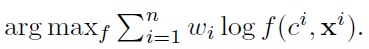
The method is particularly efficient and easy to implement in that searching for a new mixture component can be done by ML learning with
Although our earlier approach was limited to fully supervised settings, in this paper we extend it to semi-supervised learning setups where we can make use of a large portion of unlabeled data points in conjunction with a few labeled data. We incorporate the minimum entropy principle in [18] into our recursive mixture estimation framework, where the unlabeled data points are exploited in such a way that the model’s uncertainty in class prediction is maximally reduced. This leads to an objective function comprising the conditional log-likelihoods on labeled data and the negative entropy terms for unlabeled data. Within the functional gradient boosting framework, we derive the stage-wise data weight distribution for this semi-supervised objective.
The paper is organized as follows. In the next two sections, we formally set up the problem and review our earlier approach to the discriminative learning of mixtures in a fully supervised setup. Our proposed semi-supervised discriminative mixture learning algorithm is described in Section 4. In the experimental evaluation in Section 5, we demonstrate the benefits of the proposed algorithms in an extensive set of time-series classification problems on many real-world datasets in semi-supervised scenarios.
Consider a classification problem where a class label is denoted by
As a classifier, the class prediction of a new observation x can be accomplished by the decision rule:
we learn a joint density
However, the ML learning does not necessarily yield optimal prediction performance unless we are given not only the correct model structure but also a large number of training samples.
The discriminative learning of BNCs effectively represents the class boundaries, and exhibits superior classification performance to ML learning that merely focuses on fitting the density to all points in the training data. CML learning, one of the most popular discriminative estimators, maximizes the conditional likelihood of
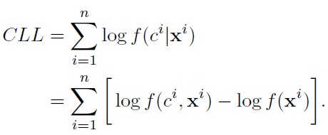
CML optimization in general does not admit closed-form solutions for most generative models. One typically maximizes it using gradient search. Although it has been shown that CML outperforms ML when the model structure is suboptimal [6,10,11,19], the computational overhead demanded by gradientbased approaches is high, especially for complex models such as HMMs and general BN structures.
1We use the notation f(c, x) interchangeably to represent either a BNC or a likelihood at data point (c, x).
3. Previous Recursive Mixture Estimation in Fully Supervised Setups
Motivated by the fact that a single BNC can be insufficient for modeling complex decision boundaries (e.g., Gaussian class-conditionals merely represent ellipsoidal clusters), one can enlarge representational capacity by forming a

Note1 that each component of the mixture is a BNC
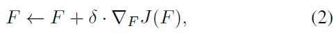
Within the functional gradient optimization framework [17], one considers how to maximize a given objective functional

Maximizing
where
Contrasting (2) with the greedy mixture update rule of (1), the optimal
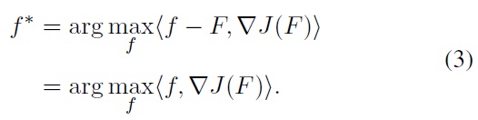
In the case of a finite number of samples
we estimate (3) as
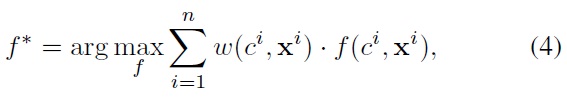
where
Once the optimal component
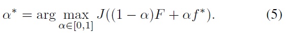
This optimization can easily be done with any line search algorithm.
It is important to discuss the choice of the objective functional
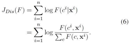
In this case, the functional gradient becomes:
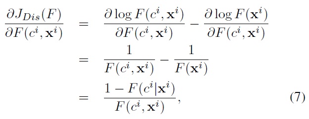
yielding the discriminative data weight:
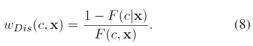
The discriminative weight indicates that the new component
The time complexity of discriminative mixture learning is of the order
1It is also worth noting that, if viewed from the generative perspective, this corresponds to modeling each class with the same number (M) of mixture components (i.e., F(x|c) for all c that have the same mixture order).
4. Semi-Supervised Recursive Discriminative Mixture Estimation
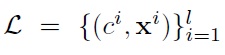
So far, we have considered the case where the data is fully labeled. In the semi-supervised setting, we are given the labeled set
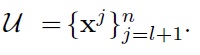
and the unlabeled data
Among several known semi-supervised classification approaches, an effective way to exploit the unlabeled data is the entropy minimization method proposed by [18]. The main idea is that we minimize the classification error for the labeled data (e.g., maximizing the conditional likelihood), while forcing the model to have minimal uncertainty in predicting class labels for the unlabeled data. This minimum entropy principle is motivated by minimization of the Kullback-Leibler divergence between the model-induced distribution and the empirical distribution on the unlabeled data that has been shown to effectively partition the unlabeled data into clusters.
Having the negative entropy term for the unlabeled data, the semi-supervised discriminative (SSD) objective can be defined as
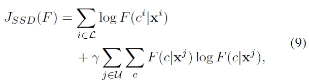
where
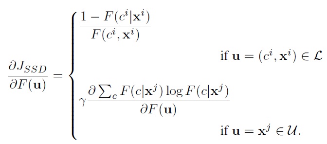
Notice that for the labeled data we have a functional gradient identical to that of supervised discriminative mixture learning. For the unlabeled data, however, the gradient terms require further consideration. The main difficulty is that for the unlabeled data x
4.1 Marginalization Over Full Label Set
A possible treatment is to assume that we are given all
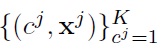
are observed in the training data. Then it follows that:
where
Hence, the unlabeled data point x
The unlabeled data weight can be interpreted as follows: (i) The denominator
Despite this intuitive interpretation, one practical issue with this weighting scheme is that the weights can be potentially negative, in which case the optimization in (4) may not be tackled by the lower bound maximization technique. In this case, one can directly optimize it using a parametric gradient search. Alternatively, the pseudo label-based technique presented next can circumvent the negative weight issue.
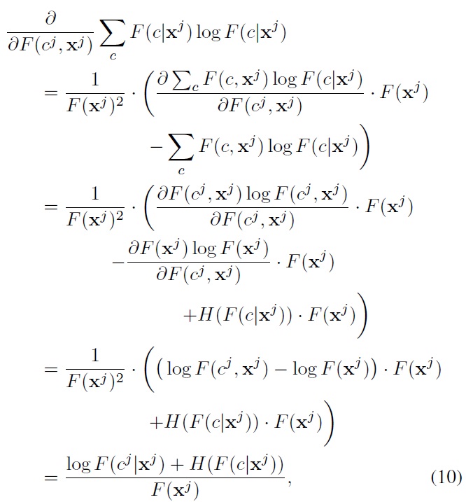
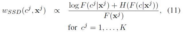
For the current model, we define the
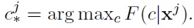
Instead of dealing with all
That is, the unlabeled x

having the following weight:
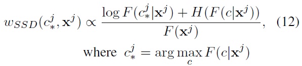
The intuition discussed in Section 4.1 follows immediately, however, we can now guarantee that the weights for the pseudolabeled data points (11) are always non-negative.
Although dealing with only the best predicted label is convenient for optimization and is a rational strategy to pursue, it is important to note that unlike the
We evaluated the performance of the proposed recursive mixture learning in semi-supervised learning settings. We focused on the structured data classification task of classifying
A simple and straightforward approach to dealing with partially labeled data is to ignore the unlabeled data points. In this section, we first summarize the fully supervised classification algorithms with which we compare our approach. These algorithms are then extended to handle unlabeled data by the wellknown and generic adaptive semi-supervised method called
The first approaches we describe are model-based, where we use (single) BNC models trained by ML and CML. In CML, the gradient search starts with the ML estimate as the initial iterate. Related to the proposed recursive discriminative mixture learning, we compare the proposed method with [21]’s
This approach has been shown to inherit certain benefits from AdaBoost such as good generalization by maximizing the margin. However, the resulting ensemble cannot be simply interpreted as a generative model since the learned BNCs are just weak classifiers to be combined for the classification task.
In addition to the model-based approaches, we also consider two alternative similarity-based approaches that have exhibited good performance in the past, especially on sequence classification problems: dynamic time warping (DTW) and the Fisher kernel [23]. DTW is a dynamic programming algorithm that searches for the globally best warping path. Often, imposing certain constraints on the feasible warping paths has been empirically shown to improve the classification performance [24-26]. For instance, the Sakoe-Chiba band constraint [24] restricts the maximum deviation of matching slices from the diagonal by
The Fisher kernel between two sequences x and x′ is defined as the radial basis function (RBF) evaluated on the distance between their Fisher scores with respect to the underlying generative model. More specifically, in binary classification,
As a baseline, we also consider a static classifier (e.g., SVM) that treats fixed-length (window) segments from a sequence as iid multivariate samples. Specifically, for a window of size

At the test stage, the class label is determined by majority voting over the predicted segment labels.
The competing methods are summarized below:
ML: ML learning of f(c, x).
CML: CML learning of f(c, x).
RDM: Recursive discriminative mixture learning [16].
BBN: Boosted Bayesian networks [21].
NN-DTW (B%): The Nearest Neighbor classifier based on the DTW distance measure where B is the best Sakoe- Chiba band constraint selected by cross validation over the candidate set: {∞%, 30%, 10%, 3%}.
FS-DTW: The function-space DTW learning [26].
SVM-FSK: The SVM classifier based on the Fisher kernel. The SVM hyperparameters are selected by cross validation. To handle multi-class settings, we perform binarization in the one-vs-rest manner. We then employ the winner-takes-all (WTA) strategy which predicts the multi-class labels by majority voting from the outputs of the one-vs-others binarized problems1.
SVM-Win (R%): An SVM classifier that treats fixedlength window segments as iid multivariate samples where R is the relative window size with respect to the sequence length (R = 100r/T). We use the RBF kernel in rd dimensional vector space. We report the best (relative) window size R selected by cross validation over a candidate set: {0% (window size r = 1), 10%, 20%, 30%, 50%}.
SSRDM: Semi-supervised recursive discriminative mixture learning (proposed approach).
In the experiments, we split the data three-fold: labeled training data, unlabeled training data, and test data. All the other approaches listed above are
We not only demonstrate the improvement in prediction performance achieved by SSRDM compared to supervised methods that ignore the unlabeled data, but we also contrast it with the generic
[Algorithm 1-1] Self-Training.
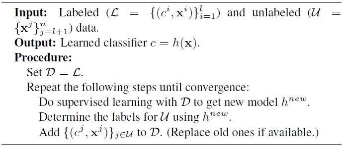
Self-Training.
Unless stated otherwise, for the mixture/ensemble approaches (i.e., BBN, RDM, and SSRDM), the maximum number of iterations (i.e., the number of BNC components) was set to ten. The test errors for the datasets (described in the next section) are shown in Table 1.
5.2.1 Gun/Point dataset
This is a binary class dataset that contains 200 sequences (100 per class) of
Weform five folds for cross validation with 10%/40% labeled/unlabeled training data and the remaining 50% for the test data, randomly . The sequences were pre-processed by Z-normalization so that the mean = 0 and standard deviation = 1. The GHMM order was chosen to be ten as it is also meaningful for describing 2?3 states for delicate movements around the subject’s side, 2?3 states for hand movement from/to the side to/from the target, 1?2 states at the target, and 2?3 states for returning to the gun holster.
The test errors (means and standard deviations) are shown in Table 1. NN-DTW with
[Table 1.] Test errors (%) for the semi-supervised settings
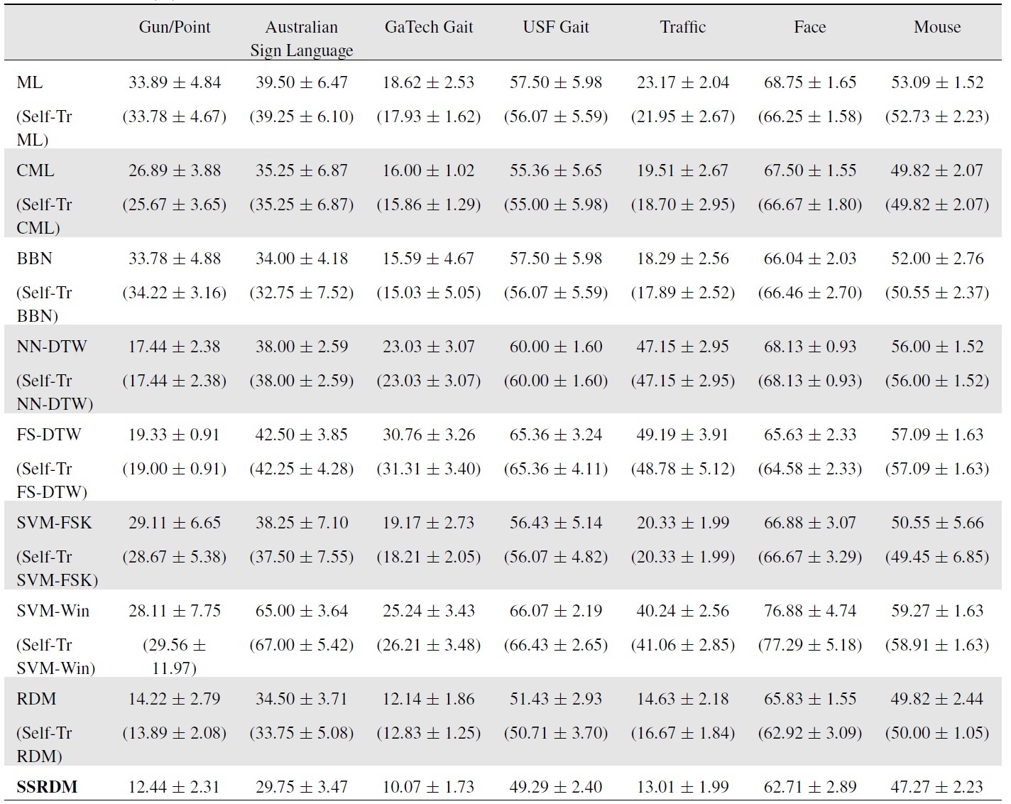
Test errors (%) for the semi-supervised settings
RDM by taking advantage of the large number of unlabeled data.
5.2.2 Australian Sign Language (ASL)
This UCI-KDD dataset contains about 100 signs generated by five signers with different levels of skill [31]. In this experiment, we considered 10 selected signs (“hello,” “sorry,” “love,” “eat,” “give,” “forget,” “know,” “exit,” “yes,” and “no”), forming a
Results in Table 1 show the test errors averaged over the five test folds. The DTW with the best-chosen band constraint (
5.2.3 Georgia-Tech speed-control gait database
We next tested the proposed mixture learning algorithms on the human gait recognition problem. The data of interest is the speed-control gait data collected by the Human Identification at a Distance (HID) project at Georgia-Tech. The database was originally intended for studying distinctive characteristics (e.g., stride length or cadence) of human gait over different speeds [32,33]. For 15 subjects, and four different walking speeds (0.7 m/s, 1.0 m/s, 1.3 m/s, 1.6 m/s), 3D motion capture data of 22 marked points (as depicted in [32]) were recorded for nine repeated sessions. The data was sampled at 120 Hz evenly for exactly one walking cycle, meaning that slower sequences were longer than the faster ones. The sequence length ranged from approximately 100 to 200 samples. Each marked point had a 3D coordinate, yielding 66 (= 22×3) dimensional sequences.
Apart from the original purpose of the data, we were interested in recognizing
After this manipulation, we randomly partitioned the data five time into 20% labeled and 50% unlabeled training data with the remaining 30% test data. The GHMM order was chosen to be three, and the maximum number of mixture learning iterations was set to 20. As Table 1 demonstrates, the proposed SSRDM again attains the lowest errors.
5.2.4 USF human ID gait dataset
The USF human ID gait dataset consists of about 100 subjects periodically walking in elliptical paths in front of a set of cameras. We considered the task of motion-based subject identification, where the motion videos were recorded in diverse circumstances: the subject walking on grass or concrete, with or without a briefcase. From the processed human silhouette video frames, we computed the 7
After randomly splitting the 112 sequences into 50% labeledtraining, 25% unlabeled-training, and 25% test sets five times, we recorded the average test errors in Table 1. The GHMM order was chosen to be three from cross validation. The maximum number of iterations for recursive mixture models was set to 20. Again, RDM and SSRDM have the lowest test errors with small variances, reaffirming the importance of the recursive estimation of discriminative mixture models when combined with the use of unlabeled data.
5.2.5 Traffic dataset
We next tackle a video classification problem that has demonstrated the utility of dynamic texture methods [34,35] in the computer vision community. Dynamic texture is a generative model that represents a video as a sample from a linear dynamical system. Dynamic texture can extract the visual or spatial components in the image measurements using PCA while capturing the temporal correlation by the latent linear dynamics. Hence, a video, potentially of varying length, can be succinctly represented by two matrices (
The dataset we used in this experiment is traffic data (also used in [36]) that contains videos of highway traffic taken over two days from a stationary camera. The videos were labeled manually as light, medium, and heavy traffic, posing a 3-class problem. The videos are around 50 frames long, where each image frame is of size (48 × 48), yielding a 2304-dimensional vector.
For the dynamic texture approach, we set the latent space dimension to be eight. We used the same dimension for our GHMM-based competing approaches, where we used the PCA dimension-reduced observation in the GHMMs. We collected 131 videos (with a nearly equal number of videos for each class), and randomly split them into 60% labeled-training, 10% unlabeled-training, and 30% test sets five times. The GHMM order was chosen to be two, and the maximum number of iterations for recursive mixture models was set to 20. The SVM classifier with the Martin distance measure estimated from the learned dynamic texture recorded a test error of 16.67 ± 1.84%, outperforming many of the competing approaches as shown in Table 1. However, the proposed SSRDM (and RDM) achieved still higher prediction accuracies than the dynamic texture model.
5.2.6 Behavior recognition
Finally, we deal with a behavior recognition task, a very important problem in computer vision. We used the facial expression and mouse behavior datasets from the UCSD vision group1. The face data are composed of video clips of two individuals, each displaying six different facial expressions (anger, disgust, fear, joy, sadness, and surprise) under two different illumination settings. Each expression was repeated eight times, yielding a total of 192 video clips. We used 96 clips from one subject (regardless of illumination conditions) as training data, and predicted the emotions of other subjects in the video clips (a 6-class problem). We further randomly partitioned the training data into 50% labeled and 50% unlabeled sets five times. The mouse data contained videos of five different behaviors (drink, eat, explore, groom, and sleep). From the original dataset, we formed a smaller set comprising 75 video clips (15 videos for each behavior). We then randomly split the data into 25% labeled training, 40% unlabeled training, and 35% test sets five times.
In both cases, from the raw videos, we extract the
For the classification, we first ran the static mixture approach in [37] as a baseline, where they represented a video as a histogram of cuboid types, essentially forming a bag-of-words representation. They then applied the nearest neighbor prediction using the
Instead of representing the video as a single histogram, we considered a sequence representation for our GHMM-based sequence models. For each time frame
The experimental results for the semi-supervised classification settings imply that SSRDM is significantly better than selftraining. This can be attributed to the SSRDM’s effective and discriminative weighting scheme that discovers the most important unlabeled data points for classification. Compared to our SSRDM, the performance improvement achieved by the self-training algorithm is small and can sometimes deteriorate classification accuracy.
1Selecting the number of hidden states in GHMMs is an important task of model selection that we accomplish using cross validation.
1Alternatively, one can directly tackle multi-class problems via multiclass SVM [27]. The other possibility in binarization is the one-vs-one treatment [28,29]. In our evaluation, however, WTA in one-vs-others settings slightly outperforms these two alternatives almost all the time, hence we only report the results of WTA.
1For further details about the data, please refer to [30].
1Available for download at http://vision.ucsd.edu.
In this paper we have introduced a novel semi-supervised discriminative method for learning mixtures of generative BNC models. Under semi-supervised settings, we utilized the minimum entropy principle leading to stage-wise data weight distributions for both labeled and unlabeled data. Unlike traditional approaches to discriminative learning, the proposed recursive algorithm is computationally as efficient as learning a single BNC model while achieving significant improvement in classification performance. Our recursive mixture learning is amenable to a pre-determined mixture order as well as robust to the choice of initial parameters.
No potential conflict of interest relevant to this article was reported.


