In this paper, we propose a formation control algorithm for underactuated autonomous underwater vehicles (AUVs) with parametric uncertainties using the approach angle. The approach angle is used to solve the underactuated problem for AUVs, and the leader-follower strategy is used for the formation control. The proposed controller considers the nonzero off-diagonal terms of the mass matrix of the AUV model and the associated parametric uncertainties. Using the state transformation, the mass matrix, which has nonzero off-diagonal terms, is transformed into a diagonal matrix to simplify designing the control. To deal with the parametric uncertainties of the AUV model, a self-recurrent wavelet neural network is used. The proposed formation controller is designed based on the dynamic surface control technique. Some simulation results are presented to demonstrate the performance of the proposed control method.
Over the last two decades, the research and development of autonomous underwater vehicles (AUVs) and surface vessels have been important issues because of their usefulness in performing missions such as environmental surveying, undersea cable/pipeline inspection, monitoring of coastal shallow-water regions, and offshore oil installations [1-5].
In addition, since performing offshore missions is more efficiently accomplished by using multiple AUVs rather than a single AUV, a large number of studies have been published concerning the formation control of multiple AUVs. There are three popular strategies in designing the formation controller: the behavior-based strategy [6], the virtual structure strategy [7-8], and the leader-follower strategy [9-11]. Among these methods, the leaderfollower method is most widely used by many researchers due to advantages such as simplicity and scalability. In the leader-follower method, the leader tracks a predefined trajectory and the follower maintains a desired separation-bearing/separation-separation configuration with the leader. The follower can be designated as a leader for other vehicles because of the scalability of formation. In addition, the leader-follower method is simple to implement since the reference trajectory of the follower is clearly defined by the leader’s movement, and the internal formation stability is induced by the control laws of the individual vehicles. A leader-follower formation controller for underactuated AUVs was proposed in [11], in which the controller needs an ”exogenous” system and this exogenous system must know each vehicle position. Skejetne proposed a formation controller such that each individual vehicle has a position relative to a point called the formation reference point [12]. However, these papers did not consider the off-diagonal terms in the system matrix or the parametric uncertainties of the AUV.
In this paper, therefore, we propose a formation control algorithm for underactuated AUVs. First, we obtain the virtual leader in reference to the follower in the leader-follower strategy; the formation problem is then dealt with as a tracking problem. Second, in order to design the controller, we use the state transformation [13], which can avoid the difficulties caused by the off-diagonal terms in the system matrix, and we employ self-recurrent wavelet neural networks (SRWNNs) [14,15] to deal with the uncertainties in the hydrodynamic damping terms. Third, using the approach angle [16] and the formation error dynamics in the body-fixed frame, we solve the underactuated problem for AUVs. Fourth, the dynamic surface control (DSC) technique [17], which can solve the ”explosion of complexity” problem caused by the repeated differentiation of virtual controllers in the backstepping design procedure, is applied to design the formation controller for underactuated AUVs. Finally, we perform computer simulations to illustrate the performance of the proposed controller.
2.1 Asymmetric Structured AUV Dynamics
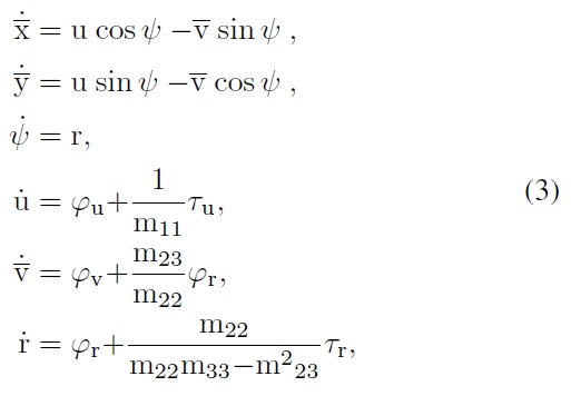
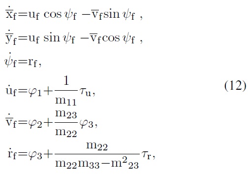
The asymmetric structured AUV has nonzero off-diagonal terms in the mass matrix, which are induced by the asymmetric shape of the bow and the stern of the vehicle. The kinematics and dynamics of the asymmetric AUV are described as follows [13]:
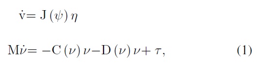
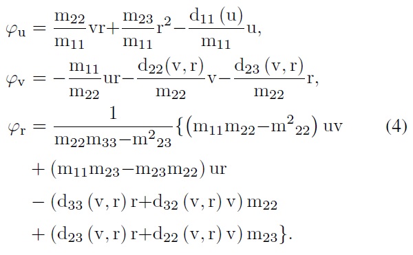
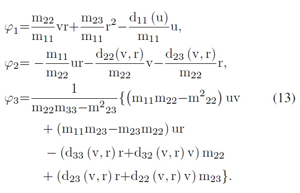
where
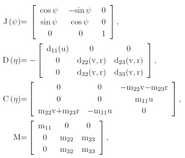
where
d22 (v, r) = ?(Yv + Yv│v│ + Yr│v│ │r│),
d23 (v, r) = ?(Yr + Yv│r│ + Yr│r│ │r│),
d32 (v, r) = ?(Nv + Nv│v│ + Nr│v│ │r│),
d33 (v, r) = ?(Nr + Nv│r│ │v│ + Nr│r│ │r│).
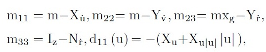
Here, Xu, Xu│u│, Yv, Yv│v│, Yr│v│, Yr, Yv│r│, Yr│r│, Nv, Nv│v│, Nr│v│, Nr, Nv│r│, and Nr│r│ are the linear and quadratic drag coefficients; m is the mass of the AUV;

Y?, and N? are the added masses; xg is the x-coordinate of the center of gravity (COG) of the AUV in the body-fixed frame; and Iz is the inertia with respect to the vertical axis.
Here the matrixMincludes the off-diagonal term m23, which is present because the shape of bow is in general different from that of stern. Therefore, the sway dynamics is are affected by the yaw moment τr because of the parameter m23. Furthermore, there are only two control inputs: the surge force τu and yaw moment τr. The number of control inputs is less than the number of degrees of freedom of the AUV in the horizontal plane. Moreover, the parameters of the AUV model (1) cannot be obtained exactly. Therefore, it is difficult to design the controller for the underactuated AUV, which has both off-diagonal terms and model uncertainties.
Since the yaw moment τr acts directly on the sway dynamics in (1), causing difficulty in designing the controller, we use the following state transformations [13]:
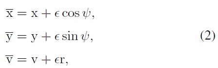
where
where
Remark 1. Here, we assume that we do not know the exact values of

and

of
2.3 Self-Recurrent Wavelet Neural Network
In this paper, we use a SRWNN to compensate for the parametric uncertainties of the AUV model. The SRWNN structure, which has Ni inputs, one output, and Ni × Nw mother wavelets, consists of four layers: an input layer, a mother wavelet layer, a product layer, and an output layer. The SRWNN output is composed of self-recurrent wavelets and parameters such that
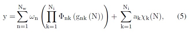
where the subscript
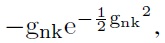
which has the universal approximation property [18]. In this paper, the five weights ak, ?nk,
The weighting vector W ∈ ?3NiNw+Ni+Nw is defined as follows:
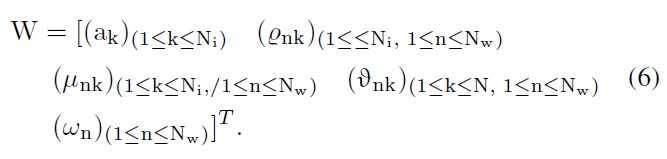
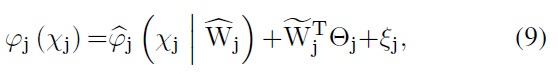
According to the powerful approximation ability [18], the SRWNN

can approximate the uncertainty term
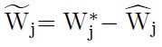
where j = u, v, r and
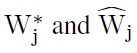
= diag(Wj), are the optimal and estimated matrices of the weighting vector of the SRWNN defined in (6), respectively, and

is the bounded reconstruction error. The optimal parameter vector

is given as
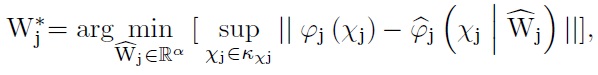
where α= 3NiNw+Ni+Nw.
Assumption 1. The optimal weight matrix is bounded such that

≤ │WMj, where ∥ㆍ∥F denotes the Frobenius norm.
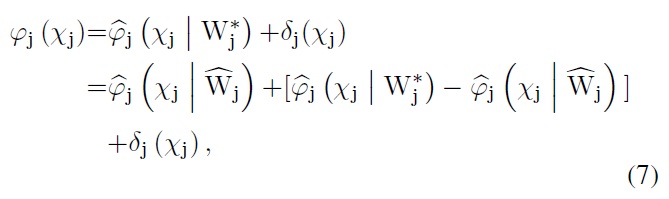
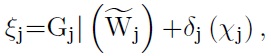
Taking the Taylor expansion of
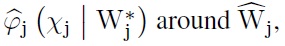
we can obtain [19].
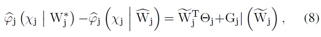
where
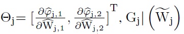
denotes the high-order terms, and
is the estimation error. Substituting (8) into (7), we have [20]
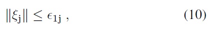
where
and ?1j>0.
By the state transformation described in subsection 2.2, the new follower’s kinematics and dynamics are as follows:
Using (11), the follower’s dynamics (11) can be rewritten as
where
According to Remark 1, the hydrodynamic parameters
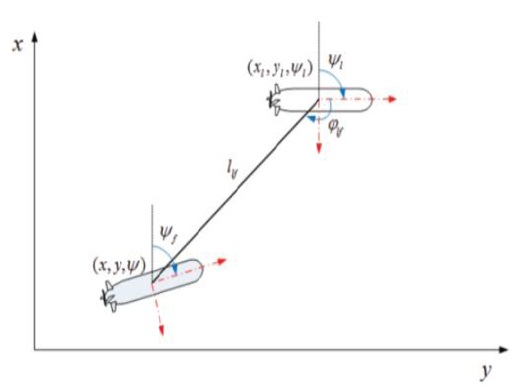
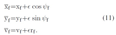
Further, to design the formation controller for underactuated AUVs, we obtain the position of the virtual reference vehicle of the followers as follows:
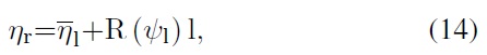
where
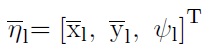
is the transformed position and yaw angle of the leader;
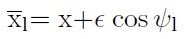
and
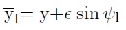
are the transformed positions of the x- and y-coordinates of the leader in the body-fixed frame;
is the desired distance between the leader and the followers; and

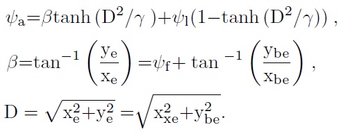
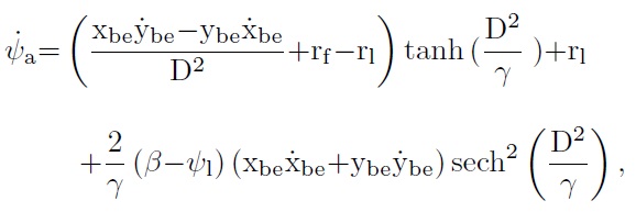
is the desired angle between the x-coordinate of the leader in the body-fixed frame and the vector from the leader to the reference vehicle as shown in Figure 1. Using the form of (1), the dynamics of
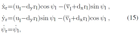
where

The reference vehicle’s dynamics (15) can be rewritten as
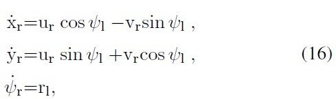
where ur=ul?dyrl and vr=vl+dxrl.
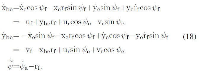
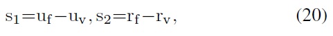
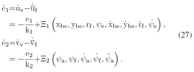
Step 1: Define the errors in the body-fixed frame as
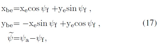
where
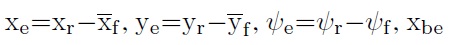
and ybe are the x- and y-coordinates of the position error in the body-fixed frame, ybe

is the yaw angle error between the approach angle
Using (16), we can obtain the following error dynamics in the body-fixed frame:
We select the virtual controls
of the follower’s surge velocity uf and the yaw velocity rf as follows:

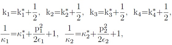
where
and k1 and k2 are the control gains to be chosen in the stability analysis.
Step 2: Define the error surface as
where the filtered signals uv and rv are obtained by passing the virtual controls
through the first-order filter as follows:

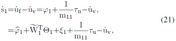
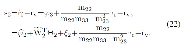
Here, k1 and k2 are positive constants. The time derivatives of s1 and s2 are then obtained as follows:
We choose the actual controls τu and τr as follows:
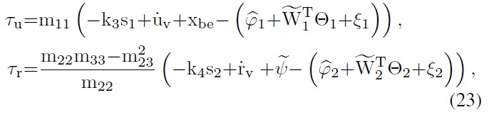
where k3 and k4 are the control gains to be chosen in the stability analysis,
are, respectively, estimates of the unknown parameters
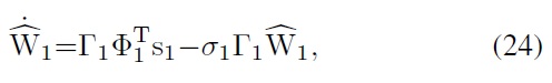
where ?1 and ?2 are positive definite matrices.
In this subsection, we show that all error signals of the closedloop control system are uniformly ultimately bounded. Define the boundary layer errors as
Then, their time derivatives are
Theorem 1. Consider the underactuated AUV (1) with parametric uncertainties controlled by (23). If the proposed control system satisfies Assumption 1, and unknown parameters
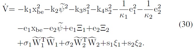
Proof. We choose the Lyapunov function as follows:
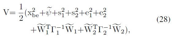
where
are positive definite matrices, and

1, 2 are the estimation errors. The time derivative of (28) along with (18), (22), (26), and (27) yields
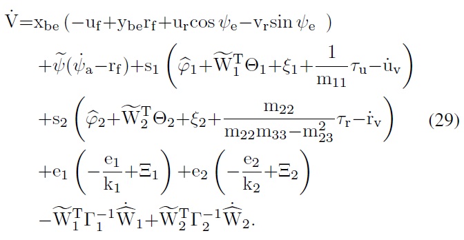
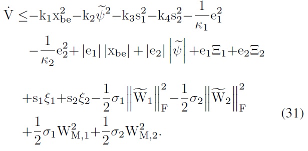
Substituting (19), (23), (24), and (25) into (29) yields
From Assumption 1, (30) can be written as
Consider a set A :=
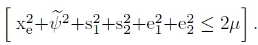
Since the set A is compact in ?7, there exist positive constants pi such
that

≤ pi, i = 1, 2. Using Young’s inequality, we have
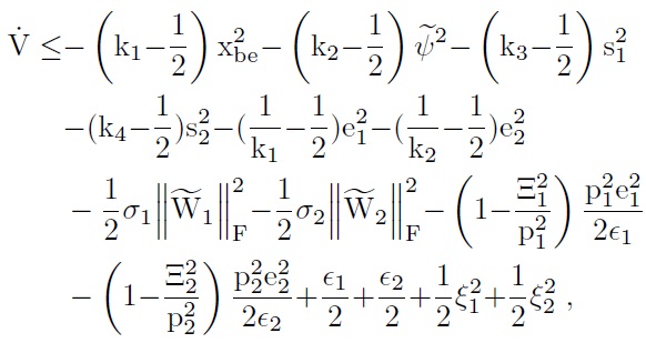
where ?i, i = 1, 2, are positive constants. If we choose
where
= 1, 2, are positive constants, then we have
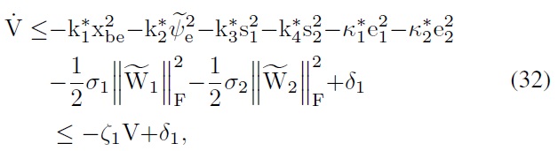
where
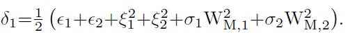
The constant
Multiplying (32) by e
Integrating (33) over [0, t] leads to
Since
In this section, we report the results of some computer simulations that illustrate the performance of the proposed formation controller for underactuated AUVs with parametric uncertainties. The surge force and the yaw moment of the leader of the AUVs are chosen as follows:
0 ≤ t ≤ 50, τul= 30, τrl= 0,
50 < t ≤ 100, τul= 30, τrl= 3,
100 < t ≤150, τul= 30, τrl= ?3,
150 < t ≤ 200, τul= 30, τrl= 0.
For the simulations, we select the initial conditions of the leader and the followers of the AUV as follows:
(xl (0) , yl (0) , Ψl (0))=(0, 0, 0) ,
(xf1 (0) , yf1 (0) , Ψf1 (0))=(?1, 0, 0) ,
(xf2 (0) , yf2 (0) , Ψf2 (0))=(?1, 0, 0)
where the subscript l indicates a leader and the subscript fi, i = 1, 2, indicates followers: xl, yl, and
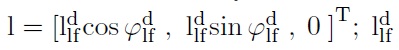
ldlf1= 2;; φdlf1= 3π/=4,
ldlf2= 2;; φdlf2= ?3π/=4.
The control gains are chosen as K1 = 0.6, K2 = 1, K3 = 2, K4 = 3, k1=1, and k2 = 1. The parameters of the SRWNN are Ni = 3, Nw = 10, and ?1 = ?2 = diag[0.1],
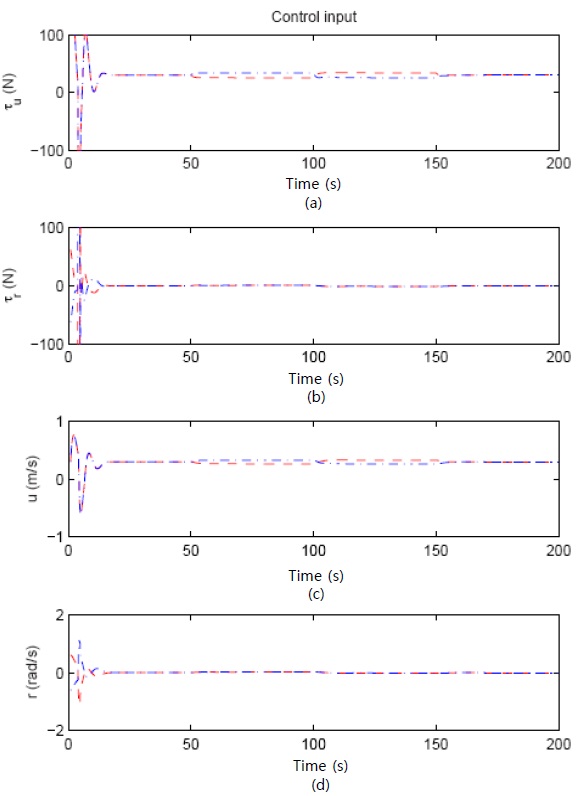
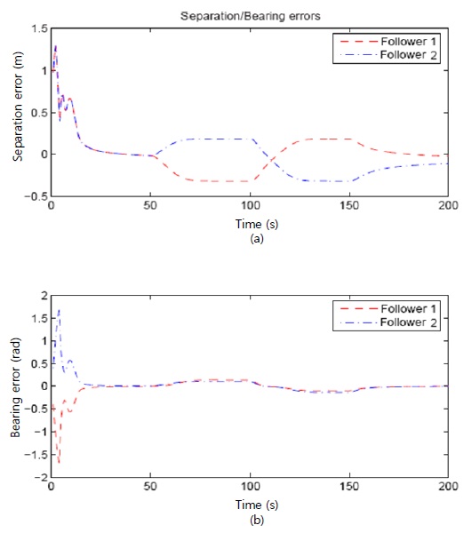
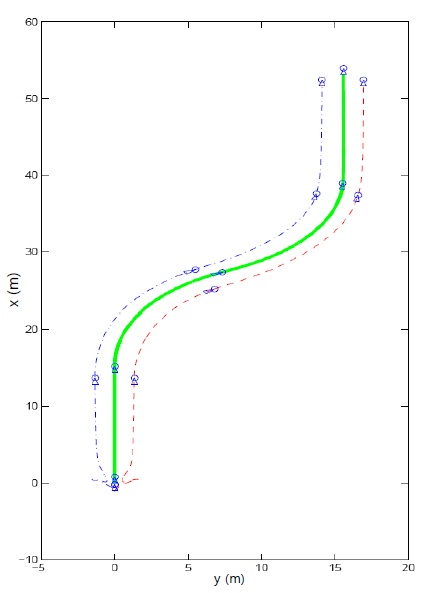
Figure 2 shows the control result of formation control for the underactuated AUVs, where the trajectory of the leader (bold line) and the trajectories of the followers (dashed line and dash-dot line) are depicted. The proposed formation control algorithm requires the followers to maintain the desired distance and angle with respect to the leader. From the result of Figure 2, the followers move along the desired position with respect to the leader at the early stage of control. Figure 3 shows the actual surge velocity u, yaw velocity r, and control inputs, which are the yaw moment τr and surge force τu. The separation and bearing errors are shown in Figure 4. Each error stays in the neighborhood of zero at the early stage of control action.
[Table 1.] Parameters of the asymmetric AUV
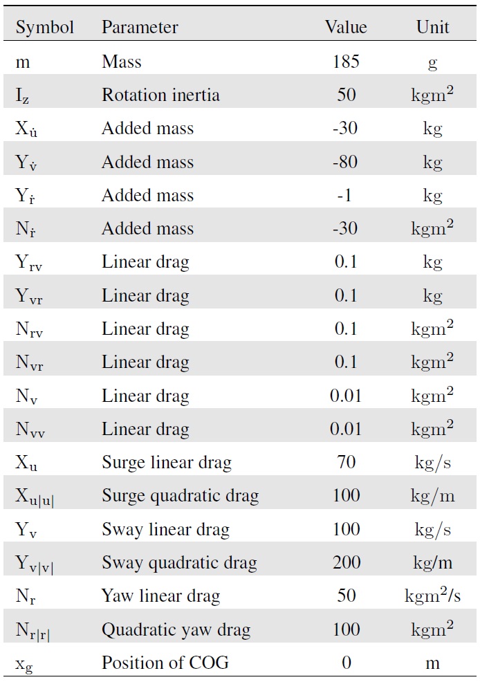
Parameters of the asymmetric AUV
We proposed a formation control algorithm for an underactuated AUV with parametric uncertainties. First, using the approach angle and formation error dynamics in the body-fixed frame, we solved the underactuated problem for AUVs. Second, the formation control algorithm was designed based on the leaderfollower strategy. Third, the state transformation was used to deal with off-diagonal terms resulting from the differences in shapes between the bow and stern. Next, the parametric uncertainties of the AUV were estimated by a SRWNN. Finally, the formation control algorithm was designed based on the DSC method. From the simulation results, we confirmed that the proposed control algorithm can maintain the predefined formation with good performance.
No conflict of interest relevant to this article was reported.