In flash radiography, the linear attenuation coefficients or the interface locations of the investigated object can be reconstructed using the information from the radiography image. However, the scattered photons in the image signal will blur the radiography or even overwhelm the useful information if there are a lot of strong scattering materials in the object. Hence, it is of great significance to estimate the scattered photons to deduct the scattering contribution.
There are many numerical methods associated with the scattering correction including the point scattered functions[1,2], Monte-Carlo scattering simulations[3], deterministic approaches for transport equation[4,5], and others[6-11]. The point scattered functions, employed by N. Kardjilov[1] and R. Hassanein[2] can improve the reconstruction accuracy for known simple geometries, but require a parameters library for point scattered functions based on different samples, different sample-detector distances, and other influencing factors. Thus, a large number of numerical calculations have to be done to obtain good results making it very time-consuming especially when the geometry and/or the material of the sample are changed. Another method is based on the Monte-Carlo simulations and has a high accuracy for arbitrary geometry. This method solves the transport processes by tracing the X-ray track, But the computing time is tremendously long due to the time-expensive stochastic Monte Carlo transport calculation method. Alternatively, the deterministic transport calculation method can also be employed to calculate the photon scattering flux by solving the Boltzmann photon transport equation. It is very difficult to find a method with both the capability of processing complex geometry and high computational efficiency.
In this paper, both the stochastic method and the deterministic method are adopted. The uncollided ray flux and the single scattered ray flux can be precisely calculated along the characteristic lines by use of the Method Of Characteristic (MOC) while the multiple scattered ray flux is corrected using numerical correction coefficients obtained through preliminary Monte Carlo simulations. Furthermore, the geometry pretreatment and ray tracing are expanded to 3-dimensional arbitrary geometry. On one hand, this coupled method overcomes the difficulties of geometric expansion experienced when using the deterministic method. On the other hand it reduces the calculation time of the multiple scattered photons and thus has a very high computational efficiency.
The remainder of this paper is organized as follows: Section 2 shows the methodology of this paper including the theoretical models of image reconstruction and scattering flux calculation, and the outline of the scattering correction during the iterative reconstruction. Section 3 analyzes the numerical results and demonstrates the reliability and capability of the method. Finally some conclusions are drawn and a few suggestions are made in Section 4.
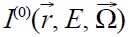
In radiographic inspection, photons arriving at the detectors can be divided into the collided and uncollided components as shown in Eq.(1).
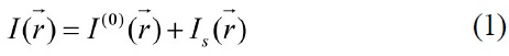
where

represents the uncollided photons,

represents the collided photons which can also be called scattered photons, and

is the spatial coordinates vector (
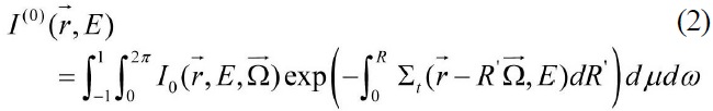
where
is the photon source,

is the direction vector,
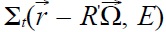
is the macroscopic cross section which is dependent on space and energy, and
The density of the object can be obtained by calculating.
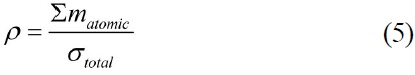
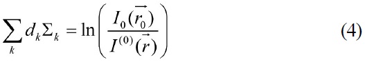
where Σ
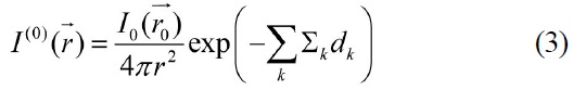
By solving equations (4) and (5), the spatial density distribution of the inspected object can be reconstructed. But in fact the reconstructed accuracy would be reduced or even distorted because the term
on the right side of Eq.(4) is disturbed by
. Especially when there are a lot of strong scatting materials in the investigated object, the scattering noise would be much bigger than the useful information. Hence, it would be very important to estimate the scattered photons to correct the scattering disturbance.
2.1 Theoretical Model of the Scattered Flux Calculation
The scattered photons can be described by the integral transport equation as shown in Eq.(6).
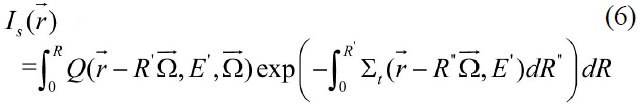
where
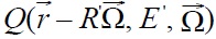
is the angular photon source,
The scattered photons can be divided into single scattered ray flux and multiple scattered ray flux as shown in Eq.(7). In this paper, the first scattered ray flux of the detectors are precisely calculated along the characteristic lines and the multiple scattered ray flux is corrected by numerical coefficients[10].
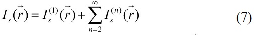
where

is the first scattered ray flux, and
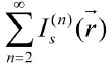
is the multiple scattered ray flux.
2.1.1. Theoretical Model of the First Scattered Ray Flux
The first term on the right-hand side of Eq.(7) is the contribution of the first scattered photons, which can be calculated using a numerical expression as in Eq.(8).
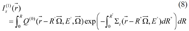
where
is the first collided photon angular scattering source.
Eq.(8) can be solved using a two-step algorithm. The first step is the spatial discretization and the computation of the scattering source for each space interval. The second step is the calculation of the scattered photons from the scattering source to the radiography image (detectors).
1) Spatial discretization
The spatial discretization is provided by ANSYS packages which can discrete the object into arbitrary geometry meshes as shown in Fig. 1. The scattering source is assumed to be continuous in each mesh and then Eq.(8) can be rewritten as
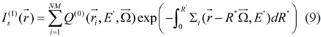
where

and
where Σ
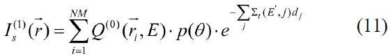
2) Angular scheme
To solve Eq.(11), the probability of the scattering source pointing to the Δ
(1) Angular scheme for Compton scattering
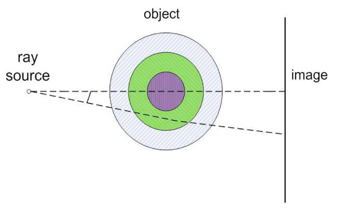
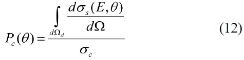
Compton scattering is a kind of strong anisotropic scattering, especially for high-energy initial photons. Most of the photons, after Compton scattering, fly forward. Fig. 2 is a schematic diagram of the Compton scattering of the ray from the photon source to the detector. The probability of the scattering source pointing to the Δθ angular region of angular θ can be expressed by Eq.(12).
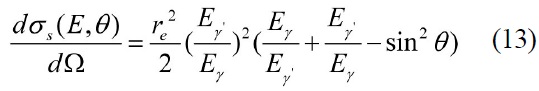
where
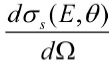
denotes the differential cross section of Compton scattering,
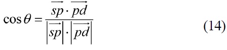
where
which can be determined by Eq.(14).
Integrating
over the 4
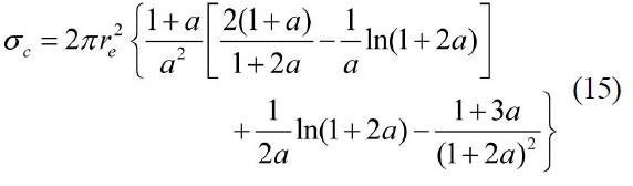
where
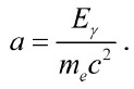
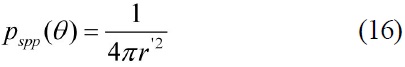
(2) Angular scheme for pair production
Considering pair production, when a photon interacts with a nucleus, an electron and a positron may be created. These particles will lose their energy during their travels in the matter. Eventually, the positron will annihilate along with other electrons by producing two photons. The energy of these two photons are both 0.511MeV and their flight vectors are exactly opposite. Based on this characteristics, pair production obeys the isotropic distribution, so the angle ratio after collision of pair production can be written as Eq.(16).
where
3) Source scheme
Eq. (17) provides the expression for the first scattered photon source
in Eq.(11).

where the first scattered photon flux for each discretized mesh obeys the exponential attenuation rule from the ray source to the mesh as shown in Eq.(18).
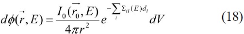
where
is the space,
is the dependent photon flux,
Because only one photon is released by the Compton effect, but two photons are released by pair production, the scattering source for Compton scattering and pair production can respectively computed by Eq.(19) and Eq.(20).
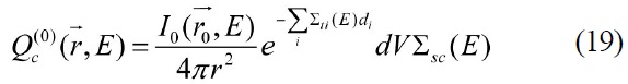
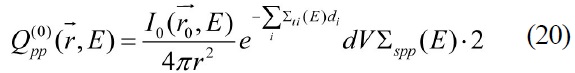
where
is the scattering source of Compton scattering,
is the scattering source of pair production, Σ
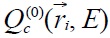
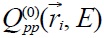
Integrating the flux contribution from all the discrete meshes to the detector, we can obtain the first scattered photon flux.
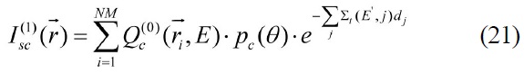
where

is the first scattered photon flux produced by Compton scattering,

is the first scattered photon flux produced by pair production. Adding these together yields the first scattered photon flux of the detector, as represented in Eq.(23).
4) Ray tracing
Based on the above theoretical model, we need to find the photon path length of each material region along the ray transport track. After geometry description and spatial discretization, ray tracing can be done. The intersections of the ray and the solid model surfaces can be searched and sorted to calculate the segment lengths in each region as shown in Fig. 3. Thus, information, including the material region number passed through, and the path length in every region, etc., can be obtained.
For an object in a known simple geometry such as a slab or spherical shell, etc., the ray tracing can be achieved accurately and efficiently, but for arbitrary geometry the geometry description, especially the ray tracing, becomes much more complicated. In the method of this paper, the ray tracing for arbitrary geometry is established using the customization of AutoCAD [12,13] to take advantage of its powerful geometric description and editing capability. This method helps to breakdown the geometry limitation into 3-dimensional arbitrary geometry, which greatly improves the capability of geometry treatment.
2.1.2 Theoretical Model of the Multiple Scattered Ray Flux
The second term on the right-hand side of Eq.(7) is the contribution of multiple scattered photons. Although its percentage compared to the total scattered flux is always small, the corresponding computation time is much longer than that of the first scattered flux. As Eq. (7) shows, there is an option to cut the multiple scattered photons off. For a sample with a long optical path, such as longer than 2 mean free paths (mfp), the ratio of the multiple scattered photons to the first scattered ones may reach up to 20% which is cannot be ignored. However, the sample contains lots of heavy media making its optical length longer than 2 mfps. Thus there is no choice but to take account of the multiple scattered flux for the sample with plenty of heavy material.
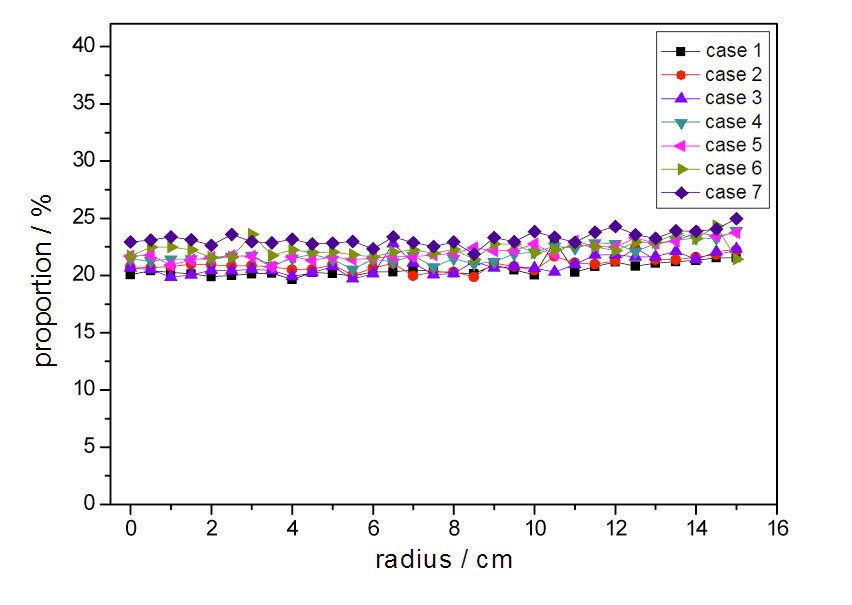
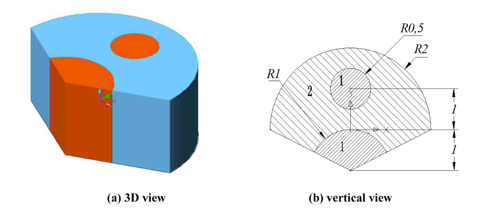
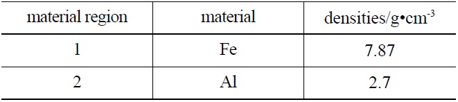
In this paper, the characteristics of the multiple scattered photons are studied in detail in terms of different parameters including geometry, material and its mass density by Monte Carlo simulations. Figure 4 shows a sample that has a spherical shell structure and contains lots of strong scattering heavy materials. By keeping the total mass constant, the geometry and the density were compressed as shown in Table 1. It can be found that the percentage of the multiple scattered photons only varies slightly with heavy changes
[Table 1.] Different Density Cases of the Object
Different Density Cases of the Object
of material mass density as shown in Fig.5. Thus it is clear that the percentage of the multiple scattered photons approximately remains the same as long as the geometry of the object does not change dramatically.
Consequently, a numerical coefficient of multiple scattered flux can be pre-calculated for the inspected sample using the Monte Carlo simulation. Then the coefficient can be used to make the correction to take account of the multiple scattered flux during the transport computation. Obviously, this can save a large amount of computational time.
2.1.3 Interpolation Method for Scattered Flux
Recently, the flat-panel detector imaging system has been employed more and more widely in 3-dimensional cone-beam flash radiography systems. For high-resolution imaging systems, there are thousands or even hundreds of thousands of pixels on each single image. Hence, it takes up a huge amount of computing time and memory if the flux of every pixel is simulated in detail. Taking the method of Monte Carlo simulations as an example, largescale workstations or even supercomputers have to be used as alternatives to a microcomputer or a PC machine to simulate the photon transporting to the flat-panel detector imaging.
In this paper, the methods of least square approximation and interpolation are used for the scattering flux calculation. Firstly, typical detectors along the radius vector in the image are selected and their detected flux is calculated. Secondly, by using the method of least square approximation, the scattered flux distribution over the image can be inputted into a function to calculate the distance between the pixel to the center of the image. Thirdly, based on the above function, the scattered flux for any pixels can been obtained by the interpolation method. This method will save a lot of computing time and memory obviously.
2.2 Scattering Correction Method
Taking the scattering effect into account as described in the previous sections, the following scattering correction and evaluation algorithm is proposed.
(1) Substituting the detected flux image into Eqs.(4) and (5) as an initial guess of the uncollided photon component yields an initial density distribution of the investigated object.
(2) Compute the scattering flux of the image, including both first and multiple scattered components, according to the information reconstructed in step (1) and the method described previously.
(3) Update the uncollided component of the flux image by subtracting the scattering contribution obtained in step (2) from the detected total photon flux.
(4) By substituting the updated uncollided photons information from step (3) into equations. (4) and (5) provides an updated density distribution can be derived.
When steps 2-4 are performed iteratively until the density distribution converges, the information of the image reconstruction will become more and more accurate.
Based on the above model, an Iterative Procedure for image restORation code (IPOR) for 3D arbitrary geometry was developed. In this section, two test problems are presented to validate the reliability and capability of the scattering correction method. Each of the two test cases includes two parts. The first part estimates the accuracy and efficiency of the scattering flux calculation method, while the second part reconstructs the density distribution of the sample. The correction effect is evaluated by comparing the results before and after scattering correction. All calculations are performed on a personal computer with an 3.2GHz Intel(R) Core™ i5 CPU. The convergence criterion for relative density error between two iterations is 10-4. Typically, the number of iterations is around 15 for those cases with heavy metal materials and less than 5 for those cases without heavy metal materials.
3.1 Case 1: Irregular 3D Cylindrical Geometry Problem
This is an irregular 3D cylindrical geometry problem as shown in Fig.6 and the height of the sample is 2 cm in
the Z direction. It contains two types of materials as shown in Table 2. The ray source is located at (0.0, -20.0,0.0) and emits photons with energy of 20MeV. The detectors are located along the plane of
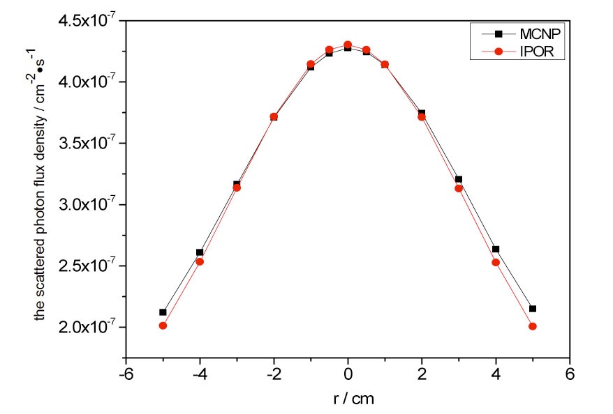
3.1.1 The Accuracy and Efficiency of the Scattering Flux Calculation Method
Fig. 7 presents the scattered fluxes of the detectors provided by IPOR and MCNP. Taking the results from MCNP as a reference, the largest relative error of IPOR is 6.7%, where the statistical estimated relative error of MCNP is in the range of 1.0 × 10⁻⁴ ~ 2.0 × 10⁻⁴. The computational time of MCNP is 153.35 minutes, but that of
[Table 2.] Material Information Data for Case 1

Material Information Data for Case 1
IPOR is only 7.99 minutes. It is demonstrated that the computational efficiency of IPOR is much higher than that of MCNP.
3.1.2 The Effect of the Scattering Correction
The density of each material region within the sample are rebuilt using the image signal of the detectors (-3.0, 20.0, 1.0) and (-3.0, 20.0, 1.0) and supposing that the initial densities are all 0.0g/cm3. Table 3 presents a comparison of the reconstructed results before and after the scattering correction. It can be seen that the scattering correction considerably reduces the error introduced during the determination of the sample densities. The largest relative error after the correction is 0.46% , which is much smaller than the error of 7.58% before the correction. It means that the application of this correction can improve the rebuilding accuracy significantly. The computing time of this case is 141.65s which is pretty short compared to the direct transport simulations.
3.2 Case 2: Spherical Shell Geometry Problem
Case two considers a spherical shell geometry problem as shown in Fig.4 and as listed in Table 4. The objective contains lots of heavy materials. In this case, the detector is a flat-panel detector with a 28 × 28 pixel
[Table 3.] The Comparison of the Reconstruction Results with and without Scattering Correction
The Comparison of the Reconstruction Results with and without Scattering Correction
array. The distance between the detector and the center of the object is 100 cm. Because the sample is rotationally symmetric, one-eighth of the image is selected to compute and study as the shaded part shown in Fig.8.
3.2.1 The Accuracy and Efficiency of the Scattering Flux Calculation Method
The reference solution is also given by MCNP. Fig. 9 shows the relative error distribution of the scattered flux in the image with the largest value of 2.9%. The statistical estimated relative error of MCNP is in the range of 1.0 × 10⁻⁴ ~ 7.5 × 10⁻³. It can been seen that IPOR provides satisfying accuracy. The computational time of MCNP is 3692.15 minutes, while that of IPOR is only 0.142 minutes. In this scenario, IPOR is superior to MCNP due to the fact that it reduces the computing time by a factor of four
[Table 4.] Material and Geometry Information Data for Case 2

Material and Geometry Information Data for Case 2
degrees of magnitude. The superiority of the computational efficiency seems much more significant in this case than in case one because in this case the detector is a flat-panel detector with 28 × 28 pixels array. All of the pixels are calculated in MCNP, but in IPOR only the selected typical pixels are calculated and the scattering distribution is obtained using least square fitting and interpolating. Thus the computational efficiency will be improved more significantly if there are more pixels in the image.
3.2.2 The Effect of the Scattering Correction
The density distribution of the sample is rebuilt based on the image signal. Fig.10 shows the radiography of this
case. It can be seen obviously that the scattered photons blur the radiographies seriously. In the region near to the center of the image, the noise overwhelms the useful information. The ratio of the uncollided photons to collided photons is presented in Fig.11. It can be found that in some regions the values are even less than 10-3. It is very difficult to reconstruct the density distribution accurately in such strong scattering situations.
The density reconstructions in terms of different scattered photons percentages are studied and the rebuilt results before and after correction are presented in Fig.12. It can be seen that the reconstruction without correction is approximately
[Table 5.] The Average Relative Error of the Reconstructed Density for the Middle Region Material
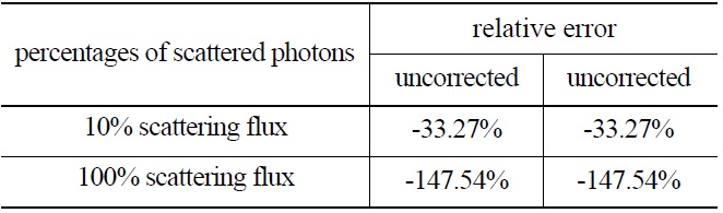
The Average Relative Error of the Reconstructed Density for the Middle Region Material
distorted for the strong scattering sample. Table 5 shows the average relative error of the reconstructed density for the middle region material and it can been seen that the rebuilding accuracy is improved by one degrees of magnitude after correction. The computing time for this case is only 160.16s.So it can been concluded that the scattering correction method not only improves the rebuilding accuracy significantly but also has a high computational efficiency.
In photon radiography, the application of scattering correction can reduce or even eliminate the disruption of the collided photons in the image, thus improving the reconstruction accuracy. The correction is based on the iterative reconstruction and scattering correction.
(1) In this paper, the uncollided ray flux and the single scattered ray flux are precisely calculated along the characteristics and the multiple scattered ray flux is corrected using numerical coefficients that have been pre-calculated. Compared with the Monte Carlo simulation, this method has both a very high computational efficiency and a satisfying accuracy.
(2) Based on the customization of AutoCAD, the geometry description and ray tracing for arbitrary geometry is carried out to greatly expand the capability of handling complex geometries.
(3) The numerical results indicate that the scattering correction can improve the reconstruction accuracy and the computational efficiency.
This scattering correction method has a high accuracy, high efficiency and expanded treatment capability for 3-dimensional arbitrary geometry. So it provides a good scattering correction method for 3D cone-beam flash radiography.