A(t), B(t), Az(t) = state-space system matrices

x(t) = state vector

u(t) = input vector

y(t) = output vector

= nominal state

？(t) = nominal output trajectories

？(t) = nominal control

= state error

ulc=u-？ = tracking error control input

M = mass of maneuvering re-entry vehicle (MaRV) exclusive of moving mass

m = mass of moving-mass element

V= velocity of MaRV

pb = relative position of mass with respect to body coordinate system

F = net aerodynamic force on twobody system

G = gravitational force on two-body system

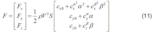
ρ = air density

S = characteristic area

α = angle of attack

β = sideslip angle

Cx0, Cxα2, Cxβ2 = resistance coefficients

Cy0, Cyα = lift coefficients

Czo, Czβ = lateral force coefficients

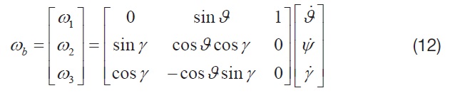
ω = angular velocity

？ = pitch angle

ψ = yaw angle

γ = roll angle

= the direction-cosine matrix from body coordinate system to ground coordinate systemg

J = moment of inertia of MaRV with respect to body coordinate system

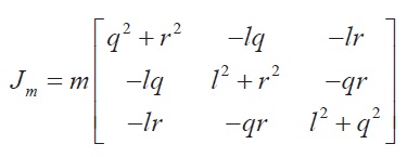
Jm = moment of inertia of moving mass with respect to body coordinate system

Ma = net aerodtnamic moment about MaRV's center of mass

L = characteristic length

= roll moment coefficients

= yaw moment coefficients

= pitch moment coefficients

μ = reduced mass parameter

ρi,k(t)(k=1, 2) = PD spectrum

ζi, ζ = constant damping

ωni(t), ω(t) = time-varting bandwidth

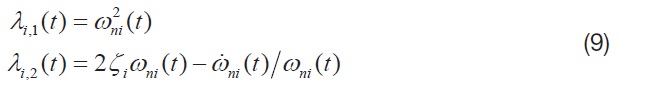
λ1, λ2 = time-varying paramenters

Superscripts:

g = ground coordinate system

b = body coordinate system

Increasing emphasis has been placed on the need for maneuvering re-entry vehicle (MaRV) designs, since future missions for atmospheric re-entry vehicles are facing the problem of a complex environment, short action time, severe weight and volume constraints on actuation and instrumentation. The simplicity of a moving-mass roll control system (MMRCS), combined with its unique ability to provide roll control from within the MaRV's protective shell, make it an attractive alternative to more traditional aerodynamic or thruster-based roll control systems [1]. The purpose of this paper is to present the roll controller using trajectory linearization control (TLC) method that can handle the uncertainties in disturbances and modeling of many modern control problems as exemplified by the controller for a MaRV.

The governing equations of motion of a coupled MaRVmoving mass two-body system are derived using the Lagrange method [2,4,5]. The mathematical model has a clear physical meaning and is free from force analysis. Classical control theories, such as PID, can barely meet the needs of MMRCS due to the nonlinearity, coupling and time-varying characteristics of the mathematical model. So modern control methods, such as optimum control [1], quadratic programming [5], and H_∞ control [6] are widely used in designing MMRCS. Although the results of the modern control methods are very attractive, the methods are unsuitable for engineering application. For example, an accurate mathematical model is essential for most modern control methods. However, the uncertainties in disturbances and modeling of an actual system may lead to degradation or failure in the controller.

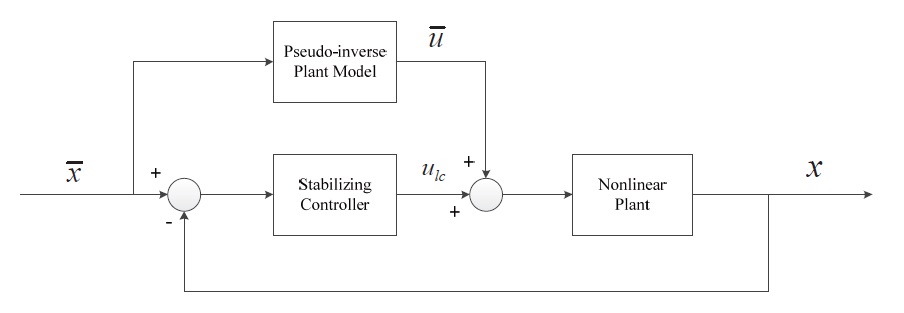
TLC is an effective nonlinear control method and it has been successfully applied in the control systems of missiles [7,8,10], robots [12] and X33 vehicle[13]. The design procedure of TLC consists of the design of two controller subsections. The first one is designed to put the vehicle on the desired trajectory by inverting the nonlinear plant. The second one is a PD-spectrum assignment controller that exponentially stabilizes the linearized tracking error dynamics. This method provides closed-loop global exponential stability without disturbances and gains the maximum robustness against disturbances. The original mathematical model of the nonlinear system is not suitable for analysis, because TLC is based on affine nonlinear systems. So the simplified roll channel dynamic equation derived from the original mathematical model is used to design the controller. Although the controller is designed only for nominal aerodynamic coefficients, excellent performance is verified by simulation for wind disturbances and variations from -30% to +30% of the aerodynamic coefficients.

Suppose the nonlinear system is described by

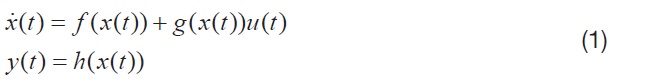
where x(t) ∈ ？ⁿ, u(t) ∈ ？^p, y(t) ∈ ？^m, f(x(t)), g(x(t)) are sufficiently smooth known vector fields of time that are bounded, and have bounded, continuous derivatives up to (n - 1) times. h(x(t)) is a smooth known function. Let

？(t), ？(t) be the nominal state, nominal output trajectories and nominal control satisfying

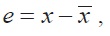
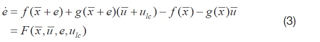
Define the state errors and the tracking error control input by

u_lc = u-？. Then the tracking error dynamics are governed by

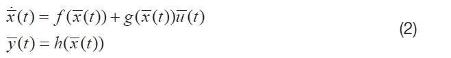
Asymptotic tracking can then be achieved by a 2 Degree-of-Freedom (DOF) controller consisting of: (i) a dynamic inverse I/O mapping of the plant to compute the nominal control function ？ for any given nominal output trajectory ？(t), of which there is a detailed discussed in Ref[11] about the pseudo-inverse and the non-minimum phase case and (ii) a tracking error stabilizing control law u_lc to account for modeling simplifications and uncertainties, disturbances and excitation of internal dynamics [9,14]. For the unperturbed system of Equation (3), exponential stability is the strongest robustness with respect to all kinds of perturbations, and it guarantees finite gain boundedinput- bounded-output stability. The structure of TLC control is illustrated in Fig. 1.

Since nominal state

and nominal input ？(t) can be regarded as additional time-varying paramenters of Equation (3), we can rewrite Equation (3) as

where

Assumption 1 Let x=0 be an exponentially stable equilibrium point of the nominal system (4), where F : [0, ∞)×D→？ⁿ is continuously cifferentiable, D = {e∈？ⁿ|？e？？r₀} and the Jaccobian matrix [∂F/∂e] is bounded and Lipshitz on D, uniformly in t. There exists a nominal control law ？ and a time-varying feedback control law u_lc such that ？=F(t, e) is locally esponentially stable.

With the assumption that the tracking errors e are small by performance requirement, the tracking error dynamics can be linearized along the nominal trajectory as

where

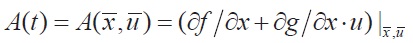
Assumption 2 The system (5), (A(t), B(t)) is uniformly completely controllable.

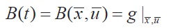
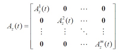
Suppose the linearized error dynamics (5) satisfy Assumption 1 and Assumption 2. Then, there exists a LTV state feedback

that can exponentially stabilize the system (5) at the origin by assigning to the close-loop system the desired PD spectrum[11], where

According to Theorem 3.11 in Ref [15], nonlinear error dynamic along the nominal trajectory is also exponentially stable at the origin. Thus, the system can be exponentially stabilized along the nominal trajectory.

The detailed design procedure and theory for PD-spectrum assignment is presented in Ref [11], along with guidelines on the selection of the closed-loop PD-spectrum. According to Theorem 3.1-5.2 in Ref [11].

where

If the subsystem

is a second-order system, the PD spectrum ρ_i,k(t)(k=1, 2) of the i-th second-order system is designed as

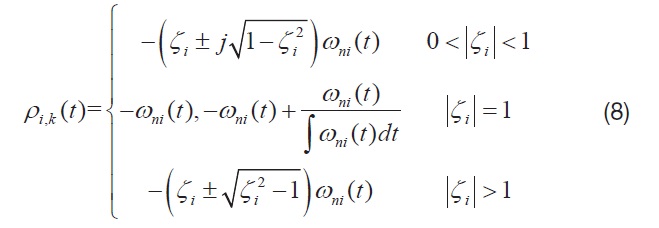
where ζ_i is the constant damping and ω_ni(t) is the time-varying bandwidth. Then the time-varying coefficients of the second-order system are

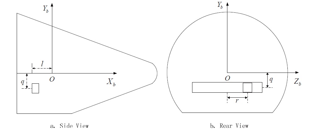
The realization of the MaRV-moving mass two-body system is shown in Fig. 2, and it consists of a cone-shaped body. The moving mass is allowed to translate with respect to the MaRV, but is not allowed to rotate with respect to the MaRV.

The system translational dynamics are given by Equation (10).

The aerodynamic force model is given by Equation (11).

The kinematic equations of attitude when the system is rolling against the centroid of the shell are given by Equation (12).

The system rotational dynamics are given by Equation (13).

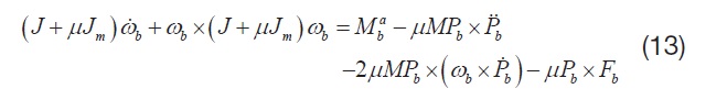
where

and the reduced-mass parameter is given by

μ=mM/(M+m)

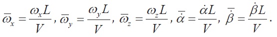
The aerodynamic moment model is given by Equation (14).

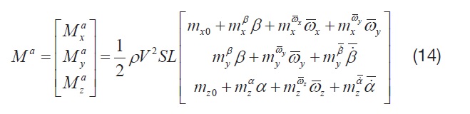
where

Equation (10) and Equation (13) describe the mathematical model of the MaRV-moving mass two-body system. See Ref [4] and [5] for the detailed derivation for the governing equations of motion.

The roll channel dynamic equation is derived according to Ref [4].

Let l=q=0 and J_s = J+μJ_m for brevity, then

Where

From Equation (12) we can get

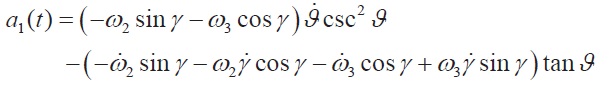
Derivate both sides of Equation (16) and substitute it into Equation (15). Then Equation (15) can be rewritten as

With further consolidation, Equation (17) is rewritten as

where

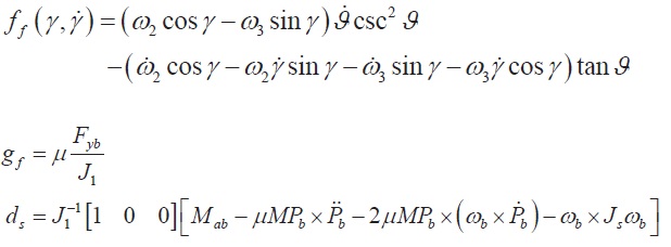
Analysis shows that the system rotational dynamic equation is non-linear, coupled and time-varying. There are also numbers of disturbling moments during the re-entry. However, the sidely used classical PD comtrol theory cannot meet the needs of MMRCS. This paper presents the attitude controller for for the roll channel using TLC.

The controller is based on the roll channel dynamic equation (18) and the desired equation ignoring the disturbance term is rewritten as

According to the design philosophy of TLC, it is essential to get the nominal control instruction of the system. The nominal control instruction of the system is the control instruction of the vehicle’s roll angle and roll angular velocity, namely

The nominal position of the moving-mass is

At the same time, to ensure causality causality,

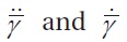
are obtained by the following pseudo differentiator

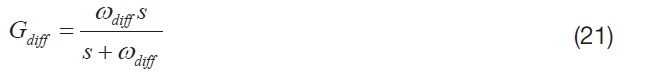
where ω_diff is the bandwidth of the low pass filter. Various factors should be comprehensively considered in choosing ω_diff, so the low pass filter can eliminate high frequency noise and allow the given control instruction.

Define the state error of system as

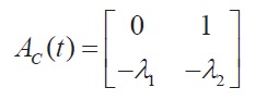
According to the design philosophy of TLC, the linearized matrix of tracking error dynamics e along

is

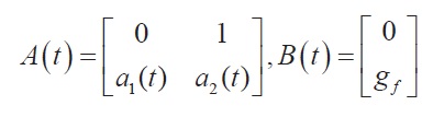
where

a2(t)=(ω2sinγ+ω3cosγ)tan？

If the desired closed-loop dynamic behavior is

Then according to

The expression of K(t) is

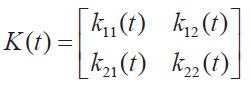
where

k11(t)=0

k12(t)=0

k21(t)=(-λ1-a1(t))/gf

k22(t)=(-λ2-a2(t))/gf

The control input of the system is

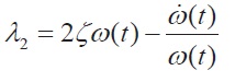
According to the pre-established PD-spectrum theory, the time-varying parameters are

λ1=ω2(t)

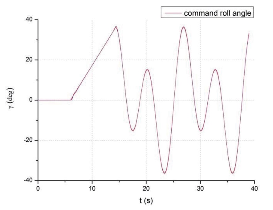
A numerical simulation of the full, nonlinear 6-DOF equations of motion is used to examine the time response of the TLC for the given roll command.

The initial conditions for the simulation are: initial speed V₀=7000m/s, initial height h₀=50km, initial flight path angle r₀=10°. The damping and time-varying bandwidth of the linear time-varying regulator are ζ=0.8 and ω(t)=50 for all the parameters used in the controller. The bandwidth of the low pass filter ω_diff is 10. The lateral position limit of the moving mass is ±0.5m.

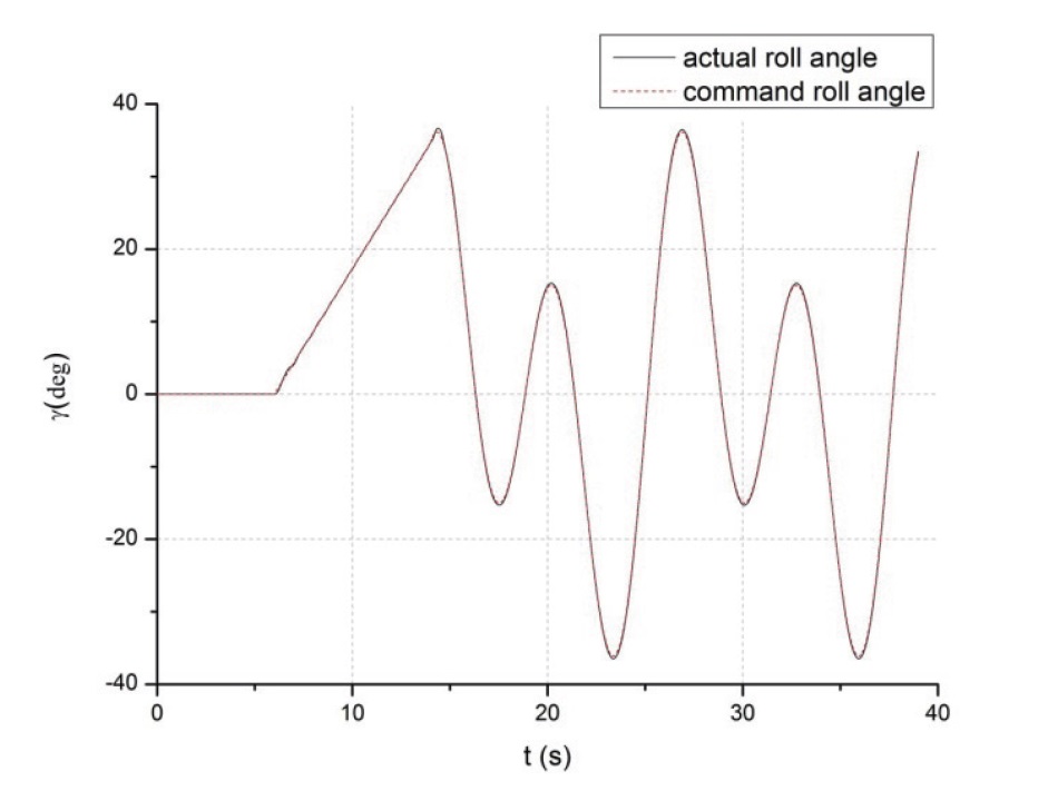
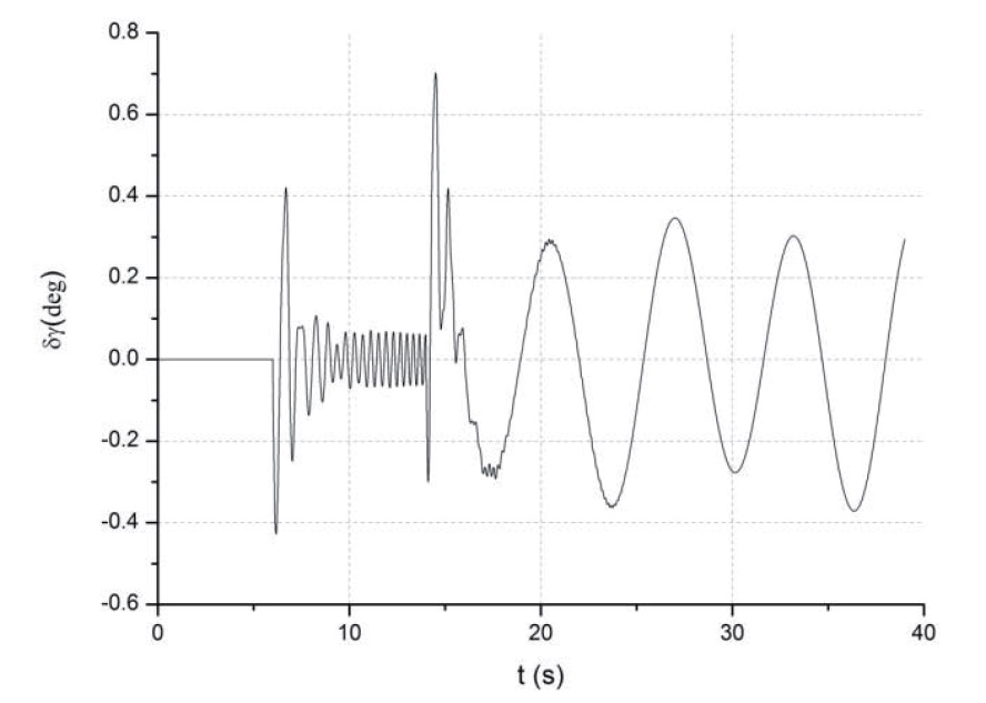
The time histories of the roll angle and tracking error are shown Fig. 3 and Fig. 4. As can be seen from the plot. the roll response is very quick with little overshoot. The maximum peak overshoot is about 0.7 degree, or 1.75% of the 40-degree commanded roll angle. Also, the tracking error is exponentially stabilized as time goes on.

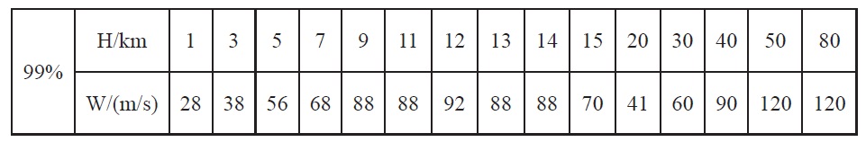
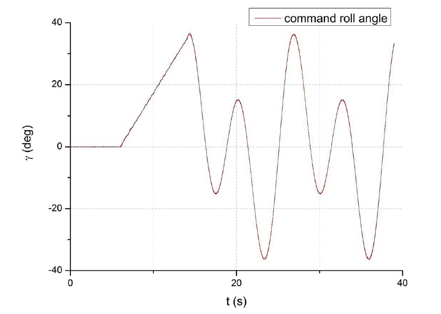
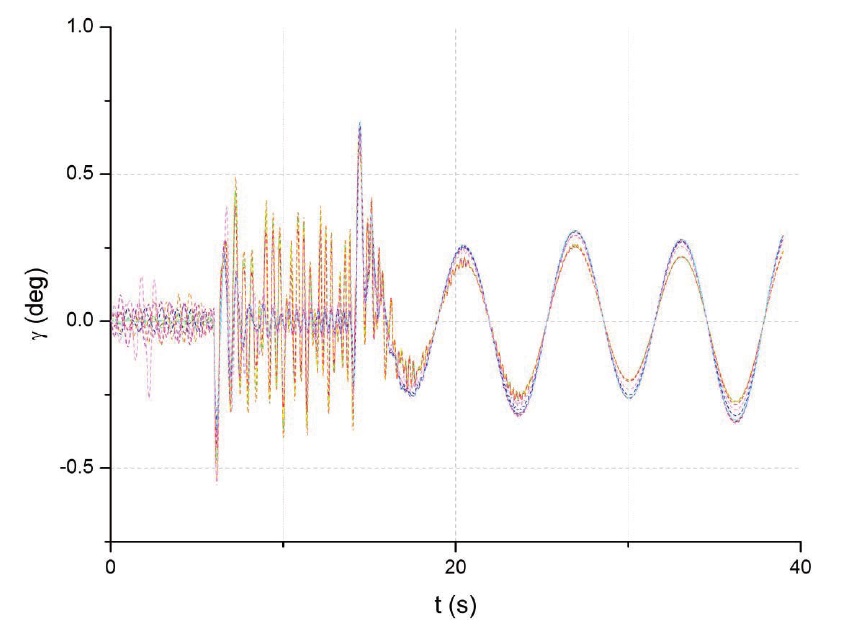
The envelope values of wind speed with a 99% probability are shown in Table 1 according to Ref[16]. Simulations are performed at the same given roll command. Fig. 5 and Fig. 6 show the responses and tracking errors of roll angle with wind disturbances.

The controller is stable when there are wind disturbances.

The maximum peak overshoot of all curves is about 0.7 degree, or 1.75% of the 40-degree commanded roll angle. Also, the tracking errors all follow the same trend when exponentially stabilized.

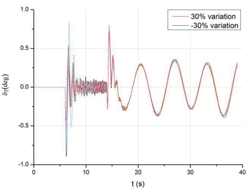
Considering ±30% variations in aerodynamic coefficients and ±10% variations in atmospheric density, the simulations are performed at the same given roll command. Fig. 7 and Fig. 8 show the responses and tracking errors of roll angle in various aerodynamic coefficients.

Obviously, the controller is still stable when there are variations in aerodynamic coefficients. The maximum peak overshoot of all curves is about 0.9 degree, or 2.25% of the 40-degree commanded roll angle. Also, the tracking errors

all follow the same trend when exponentially stabilized.

This paper presented a nonlinear, time-varying controller design for an MaRV using the trajectory linearization method. The nonlinearity, coupling and time-varying characteristics of the MaRV pose great challenges to the controller and TLC provides a satisfactory solution for the MMRCS. The controller structure exhibits considerable inherent robustness and decoupling capability without high actuator activity, providing a useful framework to deal with MaRV problems. Simulation shows that the controller is capable of dealing with different instructions. Although the controller is designed only for nominal aerodynamic coefficients, excellent performance is verified for wind disturbances and ±30% variations of the aerodynamic coefficients. It is this “plug-and-play” feature that is highly preferential for developing, testing and routine operating of the re-entry vehicles.

Future research plans include improving controller performance by: (i) using a nonlinear observer to take advantage of the ignored disturbance term d_s for a better output-feedback and (ii) ω_i(t) is a time-varying coefficient and time variation bandwidth (TVB) method should be taken into account. In particular, (i) should prove effective in overall tracking performance.