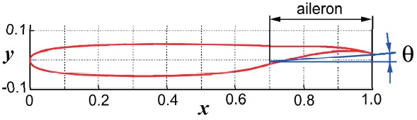
검색 전체 메뉴
PDF
맨 위로
OA 학술지
Transonic flow past a Whitcomb airfoil with a deflected aileron
  • 비영리 CC BY-NC
  • 비영리 CC BY-NC
ABSTRACT
Transonic flow past a Whitcomb airfoil with a deflected aileron
KEYWORD
Local supersonic regions , Aileron deflection , Instabilitym Lift coefficient
  • 1. Introduction

    The correct prediction of the effectiveness of wing control surfaces (ailerons and spoilers) is of major importance in the process of aircraft design. The development of numerical methods enables accurate simulation of transonic flow over control surfaces with fixed deflection angles [1,2]. A number of studies examined transonic flow over time-dependent flaps, as well as aeroelastic behavior of airfoils and wings [3-5]. However, the flow sensitivity to small perturbations in various bands of the angle of attack and Mach number has not been subject to detailed analysis.

    The upward deployment of an aileron or spoiler flattens the profile in the vicinity of the aileron-airfoil juncture or even makes it locally concave. In the 2000s, a number of numerical studies demonstrated a high sensitivity of transonic flow to variations of free-stream parameters when the airfoil comprises a flat or nearly flat arc. The sensitivity is caused by the interaction of two supersonic regions that arise and expand on the arc as the free-stream Mach number increases. The expansion followed by a coalescence of the supersonic regions crucially changes pressure distributions and aerodynamic loads on the airfoil. This phenomenon was scrutinized for a number of symmetric profiles [6-7], as well as for the asymmetric J-78 airfoil whose upper surface is nearly flat in the midchord region [6,8]. Also the instability of closely spaced supersonic regions was examined for a Whitcomb airfoil with a deflected aileron at the Reynolds number Re=5.6×10⁶ [9].

    In this paper, we study transonic flow past a Whitcomb airfoil with aileron deflections at the vanishing or negative angles of attack, which are typical for a descending flight of civil and transport aircraft, at Re=1.4×10⁷. The emphasis is laid on the flow physics and free-stream conditions that admit anomalous behavior of the lift coefficient.

    2. Problem formulation

    We consider a fully turbulent 2D flow past an airfoil given by the expressions

    image
    image

    where x and y are non-dimensional Cartesian coordinates, and ywhit(x) refers to the Whitcomb integral supercritical airfoil [10]. The last term in (1b) shifts the rear part of the airfoil upward, simulating an aileron rotation at a small angle θ, as illustrated in Fig. 1. The airfoil is placed at the center of a lens-type computational domain, bounded by two circular arcs, Γ1: x(y)= 105?(1452 ? y2)1/2 and Γ2: x(y)= ?105+(1452 ? y2)1/2, ?100≤ y ≤ 100. The width and height of the domain are 80 and 200, respectively. We set the length Lchord of the airfoil chord to 2.5 m.

    On the inflow part Γ1 of the boundary, we prescribe stationary values of the angle of attack α, free-stream Mach number M?1, and static temperature T=223.15 K. On the outflow boundary Γ2, we impose the static pressure p=26,434 N/m2. The above values of T and p are respective to the standard atmosphere at a height of 10 km. The noslip condition and vanishing flux of heat are used on the airfoil. The air is assumed to be a perfect gas whose specific heat at constant pressure is 1004.4 J/(kg K) and the ratio of specific heats is 1.4. We adopt the value of 28.96 kg/kmol for the molar mass, and use the Sutherland formula for the molecular dynamic viscosity. Initial data are parameters of the uniform free-stream, in which the turbulence level was set to 0.2%.

    3. A numerical method

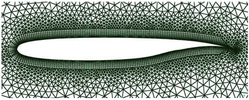
    Solutions of the RANS equations were obtained with the ANSYS 13 CFX finite-volume solver based on a highresolution discretization scheme for convective terms [11]. We employed an implicit second-order accurate backward Euler scheme for the time-stepping. Computations were performed on hybrid unstructured meshes of about 4×10⁵ cells, which were clustered in the boundary layer, in the

    wake, and in the vicinities of the shock waves. The nondimensional thickness y+ of the first mesh layer on the airfoil was less than 1 (see Fig. 2). We used the standard k-ω Shear Stress Transport turbulence model, which reasonably predicts aerodynamic flows with boundary layer separations from smooth surfaces [12].

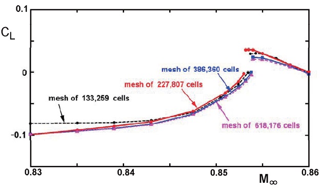
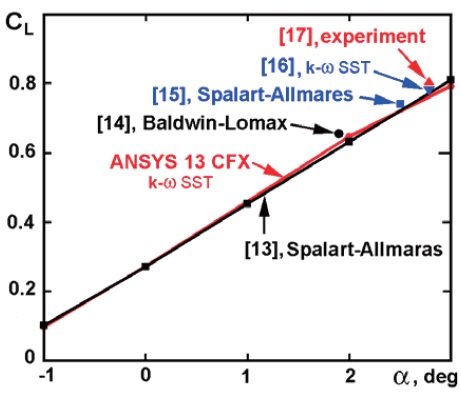
    The solver was verified by computation of solutions for a few benchmark problems and comparison with experimental and numerical data available in the literature. Figure 3 shows good agreement of the lift coefficient CL(α) calculated for a RAE 2822 airfoil at ?1≤α, deg≤3 with results obtained in [13-17]. Also the solver was used for the simulation of an oscillatory transonic flow past a 18% thick circular-arc airfoil at zero angle of attack and Re=1.1×10⁷. The amplitude of lift coefficient oscillations at M=0.75 was 0.35. This agrees well with the value of 0.37 obtained numerically in [18] using the Spalart-Allmaras and Baldwin- Lomax turbulence models.

    4. Results and discussion

    In the case of stationary boundary conditions, steadystate solutions were obtained by the global time-stepping in 2 to 6 seconds. The solutions yield a flow field, as well as aerodynamic forces on the airfoil. This makes it possible to calculate the lift coefficient CL=2FU2 S), where F is the normal force, U is the free-stream velocity module, and S is the wing area in plaform. For the simulation of 2D flow we used 3D meshes with one cell of length Lz=0.01 m in the z-direction, so that S=Lchord×Lz=0.025 m2. Figure 4 displays plots of the lift coefficient versus m calculated on three different meshes at the angle of attack α=-0.8 deg and the aileron deflection angle θ=4 deg. Evidently, the mesh of

    386,360 cells provides a good accuracy of the solution.

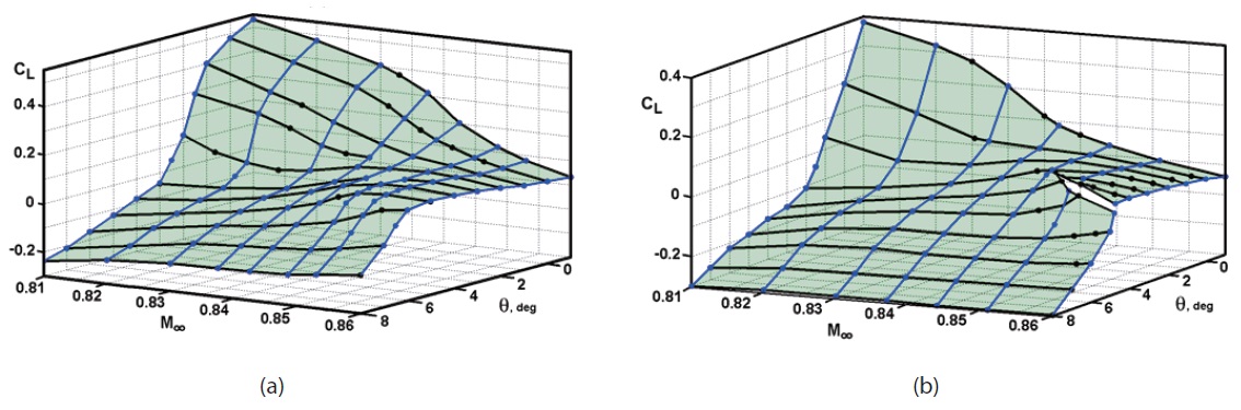
    Figure 5 illustrates the obtained dependence of the lift coefficient CL on two parameters, M and θ, for airfoil (1) at the angles of attack α=0 and α= ?0.8 deg. As seen from Fig. 5a, if α=0 and M ? 0.838, then a deflection of the aileron from zero to three degrees entails a considerable fall of the lift coefficient. This is caused by a rapid shrinking of the supersonic region on the upper surface and expansion of the supersonic region on the lower surface of the airfoil. If α=?0.8 deg, then abrupt changes of CL take place at larger values of M and 3.5 ? θ, deg ?5, so that the surface CL(M,θ) comprises a slit at 0.846< M ≤0.86 (see Fig.5b)

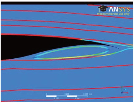
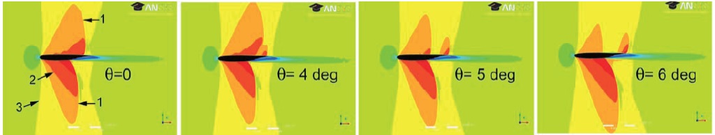
    At the same time Figs. 5a and 5b show that, when M?0.855, the lift coefficient is independent of aileron deflections up to 5 and 4 degrees, respectively. This can be explained again by the interplay of local supersonic regions. Indeed, Figure 6 shows that at θ=0 the airfoil’s trailing edge resides in a stagnation zone above the streamline separated from the lower surface of the airfoil. That is why moderate upward deflections of the aileron do not influence the flow field. With increasing aileron deflection angle from 0 to 4 deg, the supersonic regions slightly expand on both surfaces (see Fig. 7), that is why the lift coefficient persists. If the angle θ further increases, then the supersonic region on the upper surface shrinks, while that on the lower surface expands. As a consequence, the static pressure drops on the lower surface, and the lift coefficient drops.

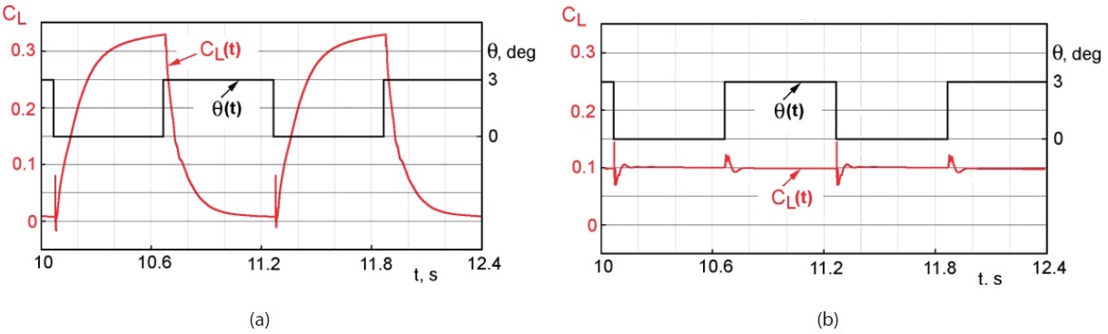
    Also we considered a time-dependent aileron deflection θ(t) that switches between 0 and 3 deg every 0.6 s, with a period of 1.2 s. Figure 8a shows a calculated dependence of the lift coefficient on time at M=0.83 and α=0. An increase of M to 0.85 results on a crucial reduction of the amplitude of lift coefficient oscillations (see Fig.8b) in accordance with Fig.5a exhibiting CL versus stationary variations of θ.

    5. Conclusions

    For the airfoil at hand, there exist adverse free-stream conditions that admit abrupt changes of the lift coefficient at small variations of the aileron deflection angle. Conversely, there exist conditions in which a response of the lift coefficient to aileron deflections is anomalously weak, so that the aileron fails to control the lift. Both anomalous phenomena are caused by the interplay of local supersonic regions on the airfoil.

참고문헌
  • 1. Henry M.M. 2001 Two-dimensional shock sensitivity analysis for transonic airfoils with leading-edge and trailingedge device deflections google
  • 2. Meheut M., Atinault O., Hantrais-Gervois J.-L. 2011 “elsA and TAU assessment for wing control surfaces” google
  • 3. Dimitrov D. 2012 “Unsteady aerodynamics of wings with an oscillating flap in transonic flow” [8th PEGASUS-AIAA Student Conference] google
  • 4. Reimer L., Heinrich R. 2013 “Modeling of movable control surfaces and atmospheric effects” [Notes on numerical fluid mechanics and multidisciplinary design] Vol.123 P.183-206 google
  • 5. Blanc F., Roux F.-X., Jouhaud J.-Ch. 2009 “Numerical methods for control surfaces aerodynamics with flexibility effects” [International Forum on Aeroelasticity and Structural Dynamics 2009] P.1-15 google
  • 6. Kuzmin A. 2012 “Non-unique transonic flows over airfoils” [Computers and Fluids] Vol.63 P.1-8 google
  • 7. Jameson A., Vassberg J.C., Ou K. 2012 “Further studies of airfoils supporting non-unique solutions in transonic flow” [AIAA Journal] Vol.50 P.2865-2881 google cross ref
  • 8. Kuzmin A. 2009 Bifurcations of transonic flow past flattened airfoils. E-print P.1-11 google
  • 9. Kuzmin A., Ryabinin A. 2012 “Airfoils admitting anomalous behavior of lift coefficient in descending transonic flight” [The Seventh Intern. Conference on Comput. Fluid Dynamics] P.1-7 google
  • 10. 1995-2013 Airfoil Coordinate Database google
  • 11. Barth T.J., Jespersen D.C. 1989 “The design and application of upwind schemes on unstructured meshes” P.1-12 google
  • 12. Menter F.R. 2009 “Review of the Shear-Stress Transport turbulence model experience from an industrial perspective” [Intern. J. Comput. Fluid Dynamics] Vol.23 P.305-316 google cross ref
  • 13. Barrett Th.R. 2007 Aerodynamic design optimization using flow feature parametrization google
  • 14. Hazra S.B. 2010 “Large-scale PDE-constrained optimization in applications”, Lecture Notes in Applied and Computational Mechanics, Vol. 49 google
  • 15. Yang J.Y., Hsieh T.-J., Huang J.C. 2010 “Implicit implementation of variant WENO schemes for compressible flow computations” [Computational Fluid Dynamics Review 2010, World Scientific] P.241-277 google
  • 16. 2006 Fluent 6.3 validation guide google
  • 17. Cook P.H., McDonald M.A,, Firmin M.C.P. 1979 “Aerofoil RAE 2822 - pressure distributions, and boundary layer and wake measurements” google
  • 18. Geissler W., Ruiz-Calavera L.P. 1999 “Transition and turbulence modelling for dynamic stall and buffet” [Engineering Turbulence Modelling and Experiments 4 (Proc. of the 4th Intern. Symposium on Engineering Turbulence Modelling and Measurements)] P.679-688 google
OAK XML 통계
이미지 / 테이블
  • [ Fig. 1. ]  Sketch of the Whitcomb airfoil with an aileron deflection at a positive angle θ.
    Sketch of the Whitcomb airfoil with an aileron deflection at a positive angle θ.
  • [ Fig. 2. ]  Sketch of the computational mesh in a vicinity of the airfoil.
    Sketch of the computational mesh in a vicinity of the airfoil.
  • [ Fig. 3. ]  Lift coefficient versus the angle of attack for a test case of transonic flow over the RAE 2822 airfoil at M∞=0.73, Re=6.5×10⁶. The references to numerical studies are accompanied by the information on turbulence models used.
    Lift coefficient versus the angle of attack for a test case of transonic flow over the RAE 2822 airfoil at M∞=0.73, Re=6.5×10⁶. The references to numerical studies are accompanied by the information on turbulence models used.
  • [ Fig. 4. ]  Convergence of the lift coefficient with mesh refinement for airfoil (1) at the aileron deflection angle θ=4 deg, angle of attack α=?0.8 deg, and Reynolds number Re ?1.4×10⁷.
    Convergence of the lift coefficient with mesh refinement for airfoil (1) at the aileron deflection angle θ=4 deg, angle of attack α=?0.8 deg, and Reynolds number Re ?1.4×10⁷.
  • [ Fig. 5. ]  Lift coefficient as a function of the aileron deflection angle θ and Mach number M∞ for transonic flow past airfoil (1) at Re ?1.4×10⁷: (a) α=0, (b) α= ?0.8 deg.
    Lift coefficient as a function of the aileron deflection angle θ and Mach number M∞ for transonic flow past airfoil (1) at Re ?1.4×10⁷: (a) α=0, (b) α= ?0.8 deg.
  • [ Fig. 6. ]  Streamlines in a vicinity of the trailing edge at M∞=0.86, α= ?0.8 deg, θ=0.
    Streamlines in a vicinity of the trailing edge at M∞=0.86, α= ?0.8 deg, θ=0.
  • [ Fig. 7. ]  Evolution of the local supersonic regions in transonic flow past airfoil (1) at the increasing angle θ of the aileron deflection and M∞=0.86, α= ?0.8 deg, Re =1.4×10⁷. Mach number contours: 1 ? M=1.0, 2 ? M=1.125, 3 ? M=0.875.
    Evolution of the local supersonic regions in transonic flow past airfoil (1) at the increasing angle θ of the aileron deflection and M∞=0.86, α= ?0.8 deg, Re =1.4×10⁷. Mach number contours: 1 ? M=1.0, 2 ? M=1.125, 3 ? M=0.875.
  • [ Fig. 8. ]  Lift coefficient as a function of time for airfoil (1) at α=0, Re?1.4×10⁷, and periodic impulse changes of the deflection angle θ: (a) M∞=0.83, (b) M∞=0.85.
    Lift coefficient as a function of time for airfoil (1) at α=0, Re?1.4×10⁷, and periodic impulse changes of the deflection angle θ: (a) M∞=0.83, (b) M∞=0.85.
(우)06579 서울시 서초구 반포대로 201(반포동)
Tel. 02-537-6389 | Fax. 02-590-0571 | 문의 : oak2014@korea.kr
Copyright(c) National Library of Korea. All rights reserved.