Optical receivers are basic building blocks in various kinds of optical communication systems. To increase the transmission distances, optical receivers suffer from various electrical and optical noises. In early optical communication systems, shot and thermal noises limit the receiver performances dominantly [1,2]. After the appearance of optical amplifiers, the amplified-spontaneous emission (ASE) becomes the most dominant noise source that mixes with the optical channel at the photo-detector [3-5]. For the analysis of optical receivers in the presence of the ASE, there are exact methods using receiver eigenmodes in the time domain [6-9] and in the optical spectral domain [10-13]. The time domain analyses have been developed initially for radiofrequency receivers.
Conventional analyses find the receiver eigenmode contributions at a specific time where the decision is made. Actually, the receiver eigenmode contributions change as a function of time within a bit period. These behaviors are affected by the optical and the electrical filters within the optical receiver. Accordingly, the distribution of the electrical voltage after the electrical filter will undergo similar changes within a pulse. Until now, however, no time-dependent analysis has been performed yet which is important for understanding the physics of optical receivers.
In this paper, we provide a time-dependent analysis of optical receivers whose optical inputs are corrupted by the ASE. We use the receiver eigenmodes in the optical spectral domain. Our analysis explains the physics about the receiver output signal and noise distributions as a function of time using receiver eigenmodes. We choose Gaussian optical receivers [14] that are good approximations to practical optical receivers yielding quantitative results with closed-form eigenfunctions.
II. TIME-DEPENDENT OPTICAL RECEIVER ANALYSYS
We assume the optical receiver has an optical filter in front of a photo-detector to select an optical channel and also to filter out the ASEs from optical amplifiers. After the photo-detector, there is a low-pass electrical filter to filter out high frequency electrical beat noises.
For simplicity, we neglect the polarization component perpendicular to that of the received signal. It will be included as an additive term after the signal contributions are fully evaluated. Just before the optical filter, the complexelectric- field amplitude is denoted as
where the kernel

We expand
where
where the asterisk symbol represents the complex conjugation.
Using (3) for (1),
The amplitude of the

Without loss of generality, we may set
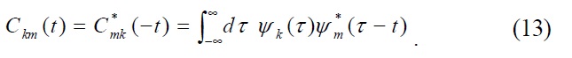
The inverse Fourier transform of (7) gives
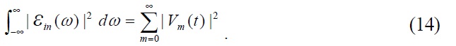
where

times the inverse Fourier transform of
Inserting (7) into (3), we find
From this relation,
where
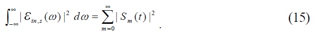
Equation (12) shows that the expansion coefficient set {
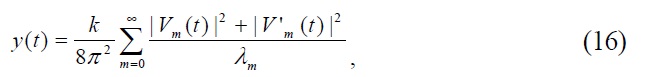
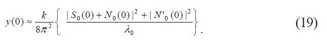
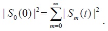
Multiplying both sides of (3) with their complex conjugates and integrating over
Equating the signal parts from both sides of (14), we have
where
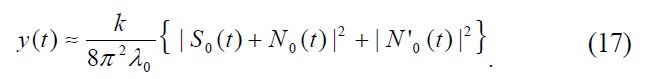
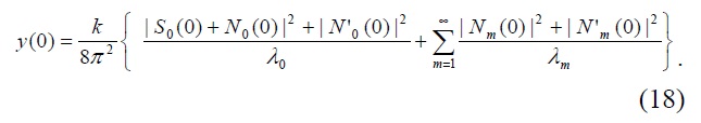
If the other polarization component of the received channel is included, (5) may be rewritten as
where we have used a prime notation for the contributions from the newly added polarization component. The polarization vector for the second term of (16) has only noise components and

[10].
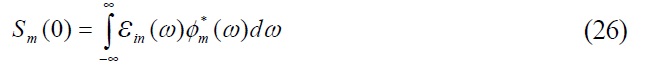
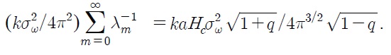
In dense wavelength-division multiplexing (DWDM) systems [15,16], the optical filter’s bandwidth is comparable to the modulation bandwidth. In this case, the magnitude of the eigenvalue
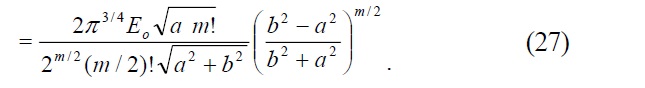
If we use
In DWDM systems, (18) may be approximated as
It is straightforward that the probability distribution function (pdf) of
Therefore, according to the central-limit theorem [19], the pdf of
III. ANALYSIS USING GAUSSIAN OPTICAL RECEIVERS
We use Gaussian optical receivers [14] for our time-dependent analysis since they are good approximations to various optical receivers and have closed form eigenfunctions. We will show that, when the received optical pulse is a Gaussian pulse, the electrical pulse after the electrical filter is also a Gaussian pulse. Then our results will be compared with our foregoing time-dependent analysis.
The optical filter of a Gaussian optical receiver has a Gaussian impulse response as

where

where

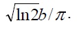
Similarly, the 3-dB bandwidth of |
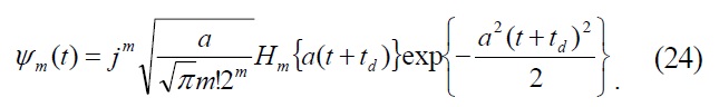
The Gaussian receiver’s eigenfunction
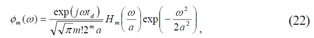
where,
The parameters,
The corresponding eigenvalues are given as
where
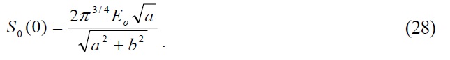
We assume the received signal is a Gaussian pulse without the ASE such that

where
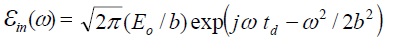
and the 3-dB bandwidth of |
When
In particular, we have for
The
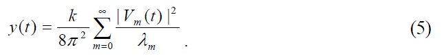
The photo-detector output current is (
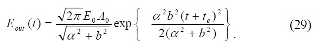
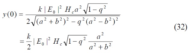
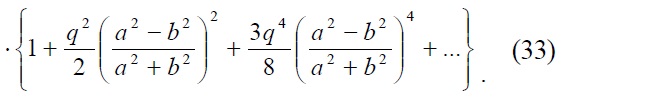
The output waveform of the Gaussian receiver for the Gaussian input (25) is also a Gaussian with its maximum at
From (5), the output of the Gaussian receiver has the following expression:
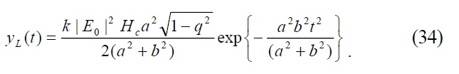
Comparing (30) with (31), we can find the receiver eigenmode contributions at arbitrary times. For example, setting

factor
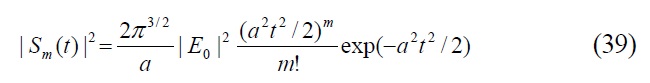
Only the even eigenmodes contribute and the lowest-order eigenmode (
We can find the lowest-order mode contribution to
factor,
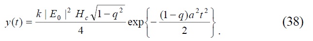
The ratio between
This ratio has a maximum at
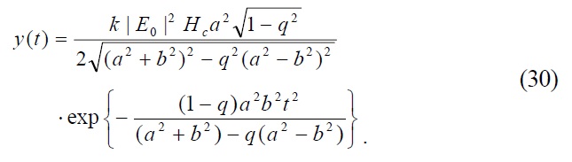
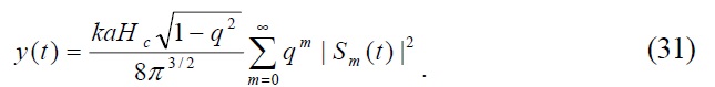
The correlation functions for the Gaussian optical receiver can be derived as
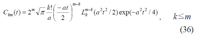
where

is the associated Laguerre polynomials [20]. Especially, when
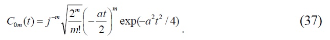
When
Comparing (38) with (31), we find
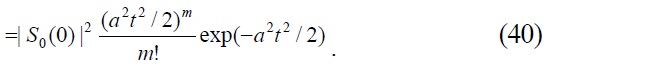
This result matches with (37).
In Fig. 1(a), we plot
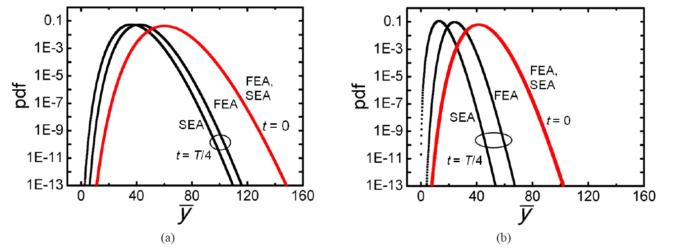
In Fig. 2(a), we show the pdfs of
We have set
as 7 GHz. At
We have analyzed the time-dependent behaviors of optical receivers corrupted by the ASE using receiver eigenmodes. The correlation functions between receiver eigenmodes in time domain determine the amplitudes of eigenmodes at different times. Gaussian optical receivers are used for our analysis that have Gaussian optical and electrical filters with closed-form receiver eigenfunctions. The edge parts of the Gaussian electrical pulse have larger contributions of higher-order eigenmodes than the pulse center where the lowest-order eigenmode is dominant. This effect is dependent on the bandwidth ratio between the optical and the electrical filters as well as the input pulse’s time width. It is enhanced when the time-width of the received Gaussian optical pulse decreases or when the bandwidth ratio increases. According to the central limit theorem, as the number of contributing eigenmodes increase, the voltage distribution of the electrical pulse at that instant becomes more symmetric and close to Gaussian. Our analysis explains the time-dependent signal and noise properties within the electrical pulses at the output of the receiver electrical filter. For Gaussian optical receivers, we have shown that the best decision time is at the peak of the electrical pulse. For other cases of non-Gaussian filters and of non-Gaussian input pulses, our analysis can be used also to get the best decision timing.