검색 전체 메뉴
PDF
맨 위로
OA 학술지
Extremely Low Numerical Dispersion FDTD Method Based on H(2, 4) Scheme for Lossy Material
  • 비영리 CC BY-NC
  • 비영리 CC BY-NC
ABSTRACT

This paper expands a previously proposed optimized higher order (2, 4) finite-difference time-domain scheme (H(2, 4) scheme) for use with lossy material. A low dispersion error is obtained by introducing a weighting factor and two scaling factors. The weighting factor creates isotropic dispersion, and the two scaling factors dramatically reduce the numerical dispersion error at an operating frequency. In addition, the results confirm that the proposed scheme performs better than the H(2, 4) scheme for wideband analysis. Lastly, the validity of the proposed scheme is verified by calculating a scattering problem of a lossy circular dielectric cylinder.


KEYWORD
Finite-Difference Time-Domain , Higher Order FDTD , Low Dispersion Algorithm , Optimization.
  • Ⅰ. Introduction

    The finite-difference time-domain (FDTD) method is an elegant way to calculate various electromagnetic phenomena due to its strengths of easy implementation and low computational quantity [1-4]. However, the standard FDTD method (the Yee scheme [5]) has a relatively large number of numerical dispersion errors when compared to other numerical analysis methods, such as the moment method and the finite element method. Many researchers have studied low dispersion algorithms in an attempt to reduce the numerical errors of the standard FDTD method [6-13].

    The higher order (2, 4) FDTD scheme (H(2, 4) scheme) is one of the low dispersion FDTD algorithms. Its weakness is that it requires a small time increment to produce accurate results, and even when a small time increment is used, its accuracy is lower than that of other low dispersion FDTD algorithms that use larger time increments at the operating frequency [11,12]. We previously presented an optimization method for the conventional H(2, 4) scheme [14]. We obtained a high level of accuracy by using the complementary dispersion properties of Yee and the H(2, 4) scheme with propagation angles, which resolved the small time increment problem of the H(2, 4) scheme. This paper expands that solution to a homogeneous, isotropic, and lossy material that has a constant conductivity for frequencies.

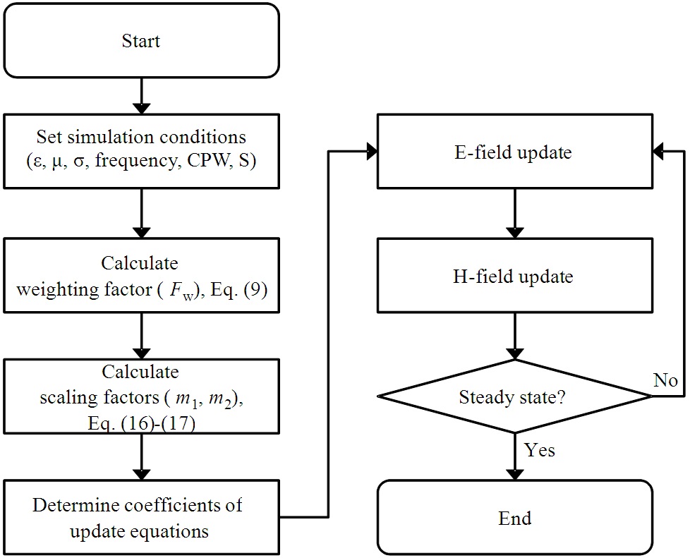
    As in our previous study [14], this study uses a weighting factor for isotropic dispersion and two scaling factors in order to achieve an extremely small number of numerical errors. However, unlike the case in the previous study [14], we use a closed-form solution in the present study to find the weighting factor. This study found a weighting factor and two scaling factors under a square grid. Fig. 1 shows the procedure of the proposed scheme. Section Ⅱ presents the formulation of the numerical dispersion relations and the calculation of a new weighting factor by a closed-form solution. The scaling factors are calculated and the scheme’s performance is analyzed in Section Ⅲ. The numerical results of the proposed scheme and the H(2, 4) scheme are compared in Section Ⅳ.

    Ⅱ. Formulation

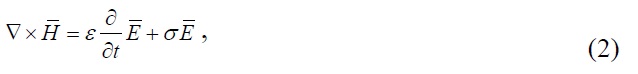
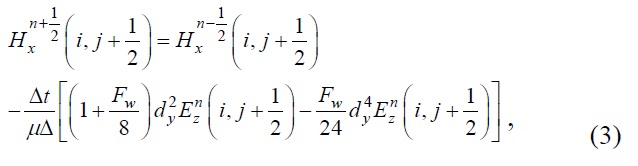
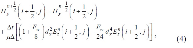
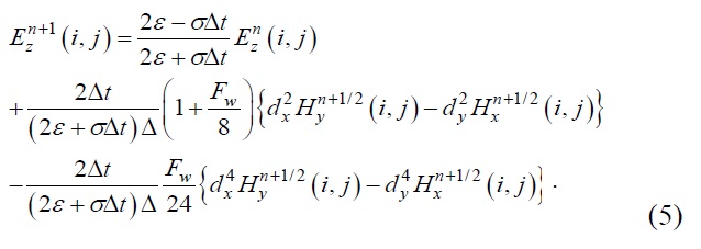
    In this section, nearly isotropic numerical phase constants for the propagation angles were obtained using a weighting factor. We assumed a square grid and found the weighting factor by using update equations and a numerical dispersion relation. The Maxwell equations used in the FDTD method are as follows:

    image
    image

    where is the electric field intensity and

    image

    is the magnetic field intensity. In addition, ε, μ, and σ are respectively the permittivity, permeability, and conductivity of a material. The following equations show the update equations of the proposed scheme at TMz-mode. A square grid ( Δ = Δx = Δy ) is assumed.

    image
    image
    image

    where

    image

    is the difference operator defined as:

    image
    image

    Fw is the weighting factor. E and H are the electric intensity and magnetic field intensity, respectively. Their subscripts indicate the field component direction. Δx and Δy denote the unit cell length of the x-direction and y-direction, respectively. Δt is a time increment. The update equations are composed of the weighting sum of the update equations of the Yee and H(2, 4) schemes. The ratio of the Yee and H(2, 4) schemes is determined by the weighting factor. If the weighting factor is one, the proposed scheme becomes the H(2, 4) scheme, and if the weighting factor is zero, the proposed scheme becomes the Yee scheme.

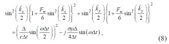
    Eq. (8) is the numerical dispersion relation of the proposed scheme.

    image

    where

    image

    is the propagation angle and c is the velocity of light. As shown in Fig. 2, the numerical phase constants of the H(2, 4) scheme and the proposed scheme have similar patterns in the propagation angles. They were obtained by Newton’s method [15]. The H(2, 4) and Yee schemes have a maximum numerical phase constant on the main axes and a minimum value on the diagonal axes. However, the phase constants of the Yee scheme are larger than the analytic phase constant, while those of the H(2, 4) scheme are smaller than the analytic value. This property makes the two schemes complementary. If the proposed scheme is used, better isotropic dispersion properties will be obtained than those of the H(2, 4) scheme.

    We determined the weighting factor (FW) using the following equation:

    image
    image

    Δβ is defined by Eq. (10) and the subscript indicates the numerical scheme (H: H(2, 4) and Y: Yee). Eq. (9) flattens the numerical wavenumbers of the proposed scheme for the propagation angles at the operating frequency.

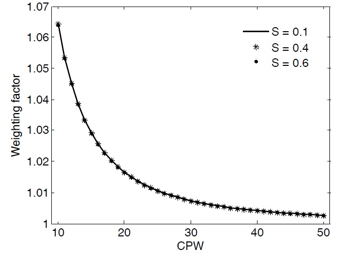
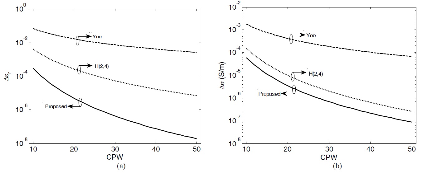
    Fig. 3 shows the weighting factor versus cells per wavelength (CPW). As shown in Fig. 3, the Courant number (S) has little effect on the weighting factor. As the CPW become larger, the weighting factor approaches a value of one. Fig. 4 shows the flatness of the relative permittivity and conductivity, defined as follows:

    image
    image

    where max(X) and min(X) stand for the maximum and minimum value of X, respectively. As shown in Fig. 4, the proposed scheme clearly has the best performance among the three schemes. Its flatness is sufficiently small to consider a constant relative permittivity and conductivity for propagation angles.

    Ⅲ. Numerical Error Reduction

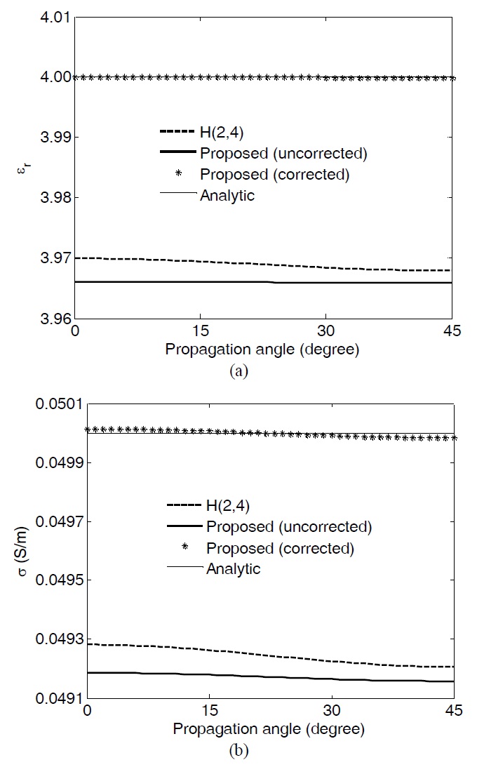
    In this section, the numerical errors are removed at a single frequency. This is followed by analysis of the wide band properties. Fig. 5 shows the relative permittivity and conductivity for the propagation angles. The estimated material constants of the proposed scheme (uncorrected) are much flatter than those of the H(2, 4) scheme. However, the difference is greater between the analytic solution and these constants than between those of the H(2, 4) scheme. These numerical errors were reduced by multiplying two scaling factors, m1 and m2, by the relative permittivity and conductivity, respectively. These create a new relative permittivity and conductivity, defined as

    image
    image

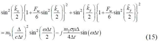
    These new material constants change the numerical dispersion relation. Eq. (15) represents the new numerical dispersion relation.

    image

    The numerical wavenumber

    image

    of Eq. (15) is changed into the exact wavenumber (k), thereby allowing analytical calculation of the scaling factors. The solution of Eq. (15) is derived as follows:

    image
    image

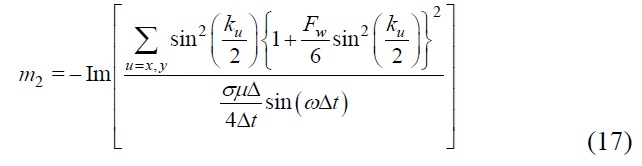
    Re[X] and Im[X] represent the real and imaginary part of X. The corrected case in Fig. 5 then represents the final performance of the proposed scheme at the operating frequency. The estimated material constants (relative permittivity and conductivity) are almost the same as the analytic values.

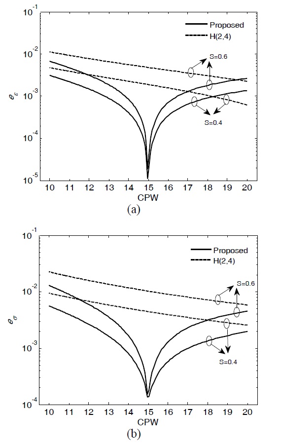
    The wideband properties of the proposed scheme are analyzed by defining
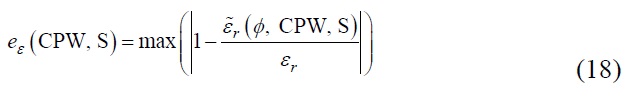
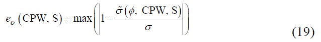
 eε(CPW, S) and eσ(CPW, S) as follows:

    image
    image

    where

    image

    are the estimated relative permittivity and conductivity, respectively. Fig. 6 the proposed scheme has a much better performance than the H(2, 4) scheme for the wide CPW region. As expected,sed scheme has an extremely small error in the selected CPW. In addition,sed scheme has similar accuracy for the different Courant numbers in the selected CPW.

    Ⅳ. Numerical Results

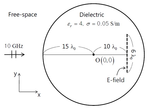
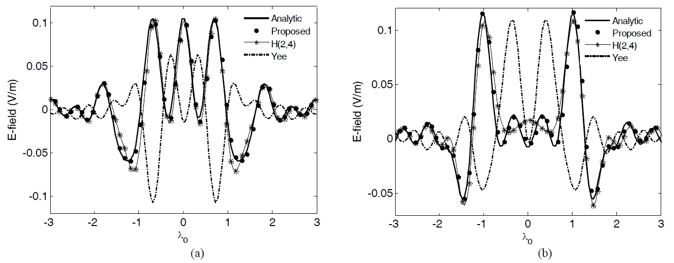
    The validity of the proposed scheme for lossy material was verified by calculating a scattering problem of the lossy circular dielectric. The radius of the dielectric is 15 λ0 at 10 GHz. The dielectric is εr =44 and σ = 0.05 S/m. A single tone plane wave is used as a source. Fig. 7 shows the simulation structure and conditions. The simulation settings are 20 CPW and 0.6 S at 10 GHz. The weighting factor and scaling factors are calculated by Eqs. (9), (16), and (17). The exact solutions were found in [8] and are compared with the calculated results. Fig. 8 shows that the results of the proposed scheme are in better agreement with the analytic solutions than are the results of the H(2, 4) and Yee schemes.

    Ⅴ. Conclusion

    In this study, we expanded the optimized H(2, 4) scheme to a lossy material and assumed a square grid. A weighting factor calculated by a closed-form solution was used to obtain isotropic dispersion in the proposed scheme. Two scaling factors were applied to the relative permittivity and conductivity and removed the numerical errors in the optimized CPW. The proposed scheme has better performance than the H(2, 4) scheme with the optimized CPW. The proposed scheme can be used effectively in electrically large problems, and can easily be expanded to 3D.
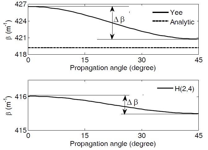
참고문헌
  • 1. Ju J. C., Lee H. Y., Park D. C., Chung N. S. 2001 "FDTD analysis of lightning-induced voltages on shielded telecommunication cable with multipoint grounding" [Journal of the Korea Electromagnetic Engineering Society] Vol.1 P.88-94 google
  • 2. Kang H. J., Choi J. H. 2002 "Full-wave analysis of microwave amplifiers with nonlinear device by the FDTD algorithm" [Journal of the Korea Electromagnetic Engineering Society] Vol.2 P.81-86 google
  • 3. Dogaru T., Le C. 2009 "SAR images of rooms and buildings based on FDTD computer models" [IEEE Transactions on Geoscience and Remote Sensing] Vol.47 P.1388-1401 google cross ref
  • 4. Wang J. B., Zhou B. H., Chen B., Shi L. H., Gao C. 2012 "Weakly conditionally stable FDTD method for analysis of 3D periodic structures at oblique incidence" [Electronics Letters] Vol.48 P.369-371 google cross ref
  • 5. Yee K. 1966 "Numerical solution of initial boundary value problems involving Maxwell's equations in isotropic media" [IEEE Transactions on Antennas Propagation] Vol.14 P.302-307 google
  • 6. Koh I. S., Kim H., Lee J. M., Yook J. G., Chang P. S. 2006 "Novel explicit 2-D FDTD scheme with isotropic dispersion and enhanced stability" [IEEE Transactions on Antennas Propagation] Vol.54 P.3505-3510 google cross ref
  • 7. Kim W. T. 2010 "Explicit isotropic-dispersion finite-difference time-domain algorithm, its characteristics and applications" google
  • 8. Kim H. 2011 "Explicit and implicit low dispersion FDTD algorithm based on isotropic-dispersion finite difference approximation" google
  • 9. Kim W. T., Koh I. S., Yook J. G. 2010 "3D isotropic dispersion (ID)-FDTD algorithm: update equation and characteristics analysis" [IEEE Transactions on Antennas Propagation] Vol.58 P.1251-1259 google cross ref
  • 10. Kim W. T., Koh I. S., Yook J. G. 2010 "3-D isotropic dispersion FDTD algorithm for rectangular grid" [IEEE Antennas and Wireless Propagation Letters] Vol.9 P.522-525 google cross ref
  • 11. Forgy E. A., Chew W. C. 2002 "A time-domain method with isotropic dispersion and increased stability on an overlapped lattice" [IEEE Transactions on Antennas Propagation] Vol.50 P.983-996 google cross ref
  • 12. Cole J. B. 1995 "A high accuracy FDTD algorithm to solve microwave propagation and scattering problems on a coarse grid" [IEEE Transactions on Microwave Theory and Techniques] Vol.43 P.2053-2058 google cross ref
  • 13. Fang J. 1989 "Time domain computation for Maxwell’s equations" google
  • 14. Oh I. Y., Hong Y., Yook J. G. 2013 "Optimization method of higher order (2, 4) FDTD method for low dispersion error" [in Proceedings of the 7th European Conference on Antennas and Propagation] P.2369-2372 google
  • 15. Taflove A. 1995 Computational Electrodynamics: The Finite- Difference Time-Domain Method. google
이미지 / 테이블
  • [ Fig. 1. ]  Flow chart for the proposed scheme. CPW=cells per wavelength, S=Courant number.
    Flow chart for the proposed scheme. CPW=cells per wavelength, S=Courant number.
  • [ Fig. 2. ]  Numerical phase constants of Yee [5], the H(2, 4) scheme and analytic phase constants. Cells per wavelength are 8 at 10 GHz and the Courant number is 0.6. The relative permittivity and permeability are 4 and 1, respectively. The conductivity is 0.05 S/m.
    Numerical phase constants of Yee [5], the H(2, 4) scheme and analytic phase constants. Cells per wavelength are 8 at 10 GHz and the Courant number is 0.6. The relative permittivity and permeability are 4 and 1, respectively. The conductivity is 0.05 S/m.
  • [ Fig. 3. ]  Weighting factor versus cells per wavelength (CPW) at different Courant numbers (S). The relative permittivity is 4 and the conductivity is 0.05 S/m.
    Weighting factor versus cells per wavelength (CPW) at different Courant numbers (S). The relative permittivity is 4 and the conductivity is 0.05 S/m.
  • [ Fig. 4. ]  (a) flatness of relative permittivity (εr=4) and (b) flatness of conductivity (σ=0.05 S/m) versus cells per wavelength (CPW). The Courant number is 0.6.
    (a) flatness of relative permittivity (εr=4) and (b) flatness of conductivity (σ=0.05 S/m) versus cells per wavelength (CPW). The Courant number is 0.6.
  • [ Fig. 5. ]  (a) Relative permittivity and (b) conductivity comparison between the H(2, 4) scheme, proposed scheme, and analytic values. Simulation settings are 10 cells per wavelength and 0.6 S at 10 GHz. S=Courant number.
    (a) Relative permittivity and (b) conductivity comparison between the H(2, 4) scheme, proposed scheme, and analytic values. Simulation settings are 10 cells per wavelength and 0.6 S at 10 GHz. S=Courant number.
  • [ Fig. 6. ]  Error comparison between the proposed and H (2, 4) schemes: (a) eε and (b) eσ . The relative permittivity is 4 and the conductivity is 0.05 S/m. S=Courant number.
    Error comparison between the proposed and H (2, 4) schemes: (a) eε and (b) eσ . The relative permittivity is 4 and the conductivity is 0.05 S/m. S=Courant number.
  • [ Fig. 7. ]  Calculation settings.
    Calculation settings.
  • [ Fig. 8. ]  Comparison of the total E-field of the proposed scheme, the H(2, 4) scheme, and the analytic solution: (a) real parts and (b) imaginary part.
    Comparison of the total E-field of the proposed scheme, the H(2, 4) scheme, and the analytic solution: (a) real parts and (b) imaginary part.
(우)06579 서울시 서초구 반포대로 201(반포동)
Tel. 02-537-6389 | Fax. 02-590-0571 | 문의 : oak2014@korea.kr
Copyright(c) National Library of Korea. All rights reserved.