Financial engineering is the field of engineering which combines the power of engineering, mathematical tools and programming in order to develop computational potency for high-performance financial trading systems [1].
Recently, most of the ongoing research in the field of finance is focused on high-performance trading and valuation using field-programmable gate array (FPGA). The super computers which were employed have become obsolete and cost ineffective as the area and power required by them is more. Earlier, better computational speed was accomplished by boosting the frequency of the microprocessor. However there are substantial limitations to this methodology which makes it impractical. Advanced microprocessors which are extremely fast need extra power and produce additional heat, which needs to be squandered.
The FPGA’s on the other hand are easy solutions with the advantage of dedicated hardware for a particular algorithm, and with tremendous reduction in area and power.
With the continuous advancements in field of FPGA, it is now easy to implement floating point arithmetic with high precision, thereby, providing the advantage of implementing complex computations faster and consuming less power and area.
In the realm of economics, computational potency directly transforms into wealth. Venture capitalists and banks employ considerable number of supercomputers to estimate and curtail risk. The Federal Deposit Insurance Corporation (FDIC) then outlines the risk weighted possessions based on these estimations. The risk weighted possessions indicates the amount of money within banks and ventures that is subjected to risk. For big corporations, this means billions which can be the total net profit of that enterprise [2].
In this paper we would discuss the hardware implementation of the European call option using Black Scholes model for financial modeling.
Financial modeling [3] pertains to the practice by which a business builds a financial model of selected, or all, attributes of the association or given collateral. A financial model is a demonstration for statistical stream of any monetary data related to any financial corporation and plays a vital role in the success and profitability of a business. It is considered as assessment and forecasting instrument for people working in the field finance especially the stock brokers, investment bankers and asset management firms. Companies spend millions of dollars in developing a model for finance, and then this model is utilized to predict the future gross and net income and evaluate various parameters such as risk and opportunity, stress, asset allocation, capital management and business planning.
Options in simple words are contract which makes the owner able enough to sell or buy an asset or stock at a certain price called as strike price and in a certain amount of time known as expiration period [3]. In order to sell off an option the owner receives a value for that option and this value which is paid by the buyer to get the right over the option is the worth of that option. The price at which an option is purchased or sold is called as premium that is the value of that option [3,4].
There are several kinds of options styles like European, Bermudan, Asian, Binary, Vanilla, Exotic, Barrier and American option [4]. The options are given different names inorder to understand the properties pertaining to specific options. The most widely used options are the European and the American options for market. The options are of many kinds like stock, bond, future contracts valuation, stock option given to an employee, real-estate options, and mutual fund options and all these options are based on two parameters known as Call and Put option price [4].
Call option is the one which gives freedom to a person to purchase an option at a certain price while a put option is the one which allows an owner to sell off an option at a certain price [3].
The option value can be divided into 2 parts:
1) Intrinsic Value
The difference between the principal price and the strike price, such that the owner of the option is at profit, is known as the intrinsic value [4]. In case of call option, the principal price of the option must be greater than the strike price of the option, hence the intrinsic value would be obtained by subtracting the strike price from principal price, while in case of a put option its reverse that is strike is greater than principal price so intrinsic value is obtained by subtracting principal price from strike price, else the intrinsic value is nil [4].
Intrinsic value (call) = current stock price ? strike price,
Intrinsic value (put) = strike price ? current stock price.
2) Time Value
The time value of an option can be defined as the value above the intrinsic value which a trader for the option. The assumption here is that before the maturity of the option the market would be bullish and worth of the assets would increase, thereby, giving profit. So, it can be observed that time to maturity is directly proportional to time value, hence, more profit considering the assumption.
Time value = option premium ? intrinsic value
The worth of the option is guided by large number of aspects like present-day worth of the option/stock, maturity time of the option that is the time of expiration, the precariousness of the cost of the holding and the selling/ purchasing price of the stock/asset which is also referred to as spot price. The method by which these attributes are affected is influenced by number of models but the flowing ones are most common [3,4]:
Monte Carlo simulation model
Binomial tree option pricing model
Black Scholes option pricing model
1) Monte Carlo Simulation Model for Option Pricing
The Monte Carlo simulation model employs Monte Carlo algorithm for the valuation of the options [5]. It computes the option value by keeping large number of uncertainty sources or the one’s which have extremely intricate characteristics.
Monte Carlo algorithm belongs to the category of mathematical algorithms which depend immensely on continuous random sampling in order to calculate the output. Monte Carlo simulation is mostly used in running big simulations of engineering and financial systems which involve extremely complex arithmetic operations. These methods require super computers due to the massive calculations involved and at times can be very slow and result in a performance hit.
A significant purpose of Monte Carlo systems in contemporary finance and risk management is in evaluating compound financial offshoots particularly when these spinoffs are based on the American style of options where the owner of the option can sell off the option even before the time to maturity [5]. For th risk management for a venture, credit of a business, market risks the Monte Carlo systems are widely used.
The option pricing valuation methodologies are inflexible, for many option styles, because the complexity involved due to the large number of variables and mathematical operations [5]. Thus Monte Carlo simulation can be extremely useful for such cases. The Monte Carlo simulation method makes use of the simulation results to estimate the random prices of the options which ultimately convert to the returns on the option. Though the method is flexible but the complexity involved is extremely high.
a) Advantages of Monte Carlo simulation
There can be only one kind of model conceivable for in-tricate systems and the analytical models are not feasible.
The simulation makes life easier as the understanding is improved because one can clearly view the real time model in simulation results
It helps in analyzing the real system, debugging it and optimizing it without operating on the actual system.
It can easily evaluate the model by varying the time while this is not possible on an actual system.
b) Disadvantages of Monte Carlo simulation
As, the various option styles involve complex differential equations, though it does not operate on the equations, but the large number of iterations involved in it makes it very slower and time consuming.
The hardware required for Monte Carlo simulation is huge, which increases the cost tremendously.
2) Binomial Tree Option Pricing Model
Binomial tree approximation, a method developed in 1979 by John Cox, Stephen Ross, and Mark Rubinstein, is also one of the most widely adopted techniques for financial modeling [4]. The most important advantage is that the me-thod does not require the use of any calculus. The method is of discrete type as compared to other models which are continuous type. So the approximation and the accuracy of the model depend on the number of time intervals taken into consideration.
When we are considering first interval of time, for example
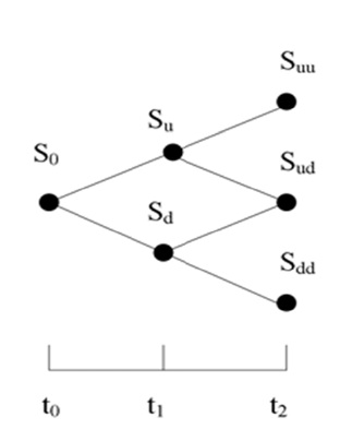
As shown in above diagram, the whole maturity time is being divided into two time intervals. In order to get from
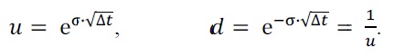
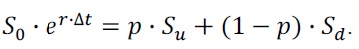
At every node, there are two possibilities. If the proba-bility of up is
The following equation also includes the risk free interest rate
Like all the models, this method has its own advantages as well as disadvantages. The Binomial method uses a relatively simpler approach. By making slight modification, method can be applied not only to European market but American market as well. Though method can be easily applied manually but for greater accuracy we need more time intervals and small step sizes. There is a need for the extra hardware. Since the method is simple, it can be easily implemented by using computer program. The method was originally developed for stock prices but because of its simplicity, the method can be applicable for calculation of dividends as well [4]. The method is relatively slower as compared to the Black Scholes method.
[Table 1.] Black Scholes and Binomial pricing model comparison [4]
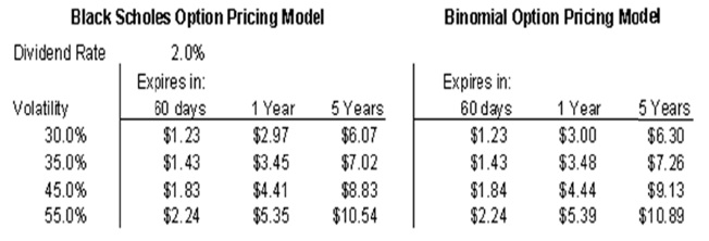
Black Scholes and Binomial pricing model comparison [4]
The method provides good approximation for the short term options. For the complicated options like that of Asian market and American market the method is inappropriate to use. The major limitation of this model is that we have to determine the step size of time. The smaller the step size more is the accuracy.
Table 1 describes the convergence between the Binomial approximation and Black Scholes method.
As one can easily analyze from the data that for the short period like 60 days, the approximation is fairly close to Black Scholes but for long period, the approximation is not valid.
So we can say that Binomial method is discrete time approximation for the Black Scholes equation which is con-tinuous time. The method is simpler and easy to implement but it shows some discrepancies from the continuous time method like Black Scholes which may lead to wrong value of call and put option and may lead to loss to individual or organization.
3) Black Scholes Option Pricing Model
The most important aspect of any hardware design is speed and cost, Black Scholes provides these privileges. As, the Black Scholes is the building block of every other model it is highly used model in today’s world. Recently, most of the ongoing research is on developing a high performance system using Black Scholes, which has led to the evolution of FPGA’s in aiding the financial modeling.
Contemporary option pricing practices are frequently con-templated amongst the critically intricate of all pragmatic areas of economics. Finance market analysts and brokers, with the advent of technology and sophisticated computing machines, are now able to calibrate the option price for a stock efficiently [4,6].
The Black and Scholes model was established in 1970 and was first enunciated in 1973 by Fischer Black and Myron Scholes in their paper which was published in the
The Black Scholes model is considered as one of the most vital theories in the field of finance and economics. It can be used to evaluate both an American and European option [4,6]. Black Scholes is considered as extremely useful for deter-mining the worth of an option whose volatility rate is extremely high.
The hardware requirement for Black Scholes system is less as compared to implementation of a Monte Carlo simulation on a FPGA and also it is faster than both the methods dis-cussed because it doesn’t require large number of iterations and the time required to set-up simulation.
III. DESCRIPTION OF ALGORITHM AND IMPLEMENTATION
The equation for call option (option which provides right to an individual to procure an option at a specific price) for Black Scholes model is as follows [4,6]:

C is the theoretical call premium,
S0 is the current price of the stock,
T is the expiration time,
K is the strike price,
r is the risk free interest rate,
N is the cumulative distribution function (CDF),
σ is the volatility of the market,
'e' is the exponential term.
In order to understand the model itself, we divide it into two parts.
The most vital part in implementation of the Eq. (1) is CDF
where,
>
A. Architecture of the Model
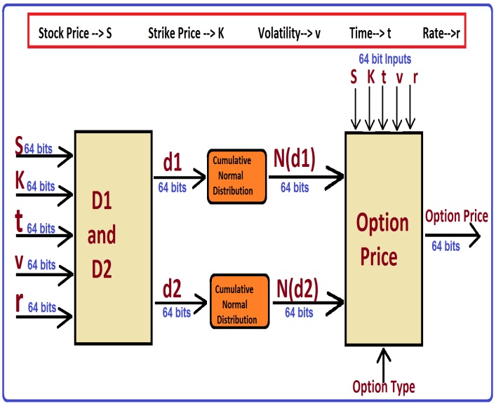
The block diagram for the Black Scholes implementation for European call option is shown in Fig. 1 on next page.
The block diagram is divided into 3 parts:
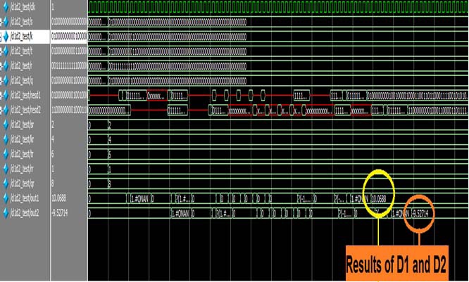
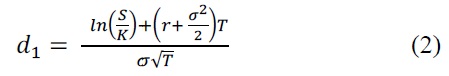
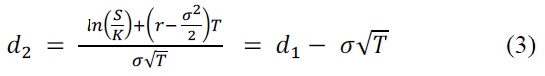
1) D1 which needs to be calculated from Eq. (2) and D2 which needs to be calculated from Eq. (3).
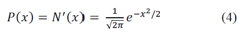
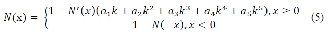
2) The 2nd block is the cumulative normal distribution, as shown in Eqs. (4) and (5), it takes the results of 1st block and performs the standard normal distribution and then CDF is finally calculated.
3) The 3rd block is the option price, the results from the cumulative normal distribution function are fed into the option price block and finally the call option value is obtained.
>
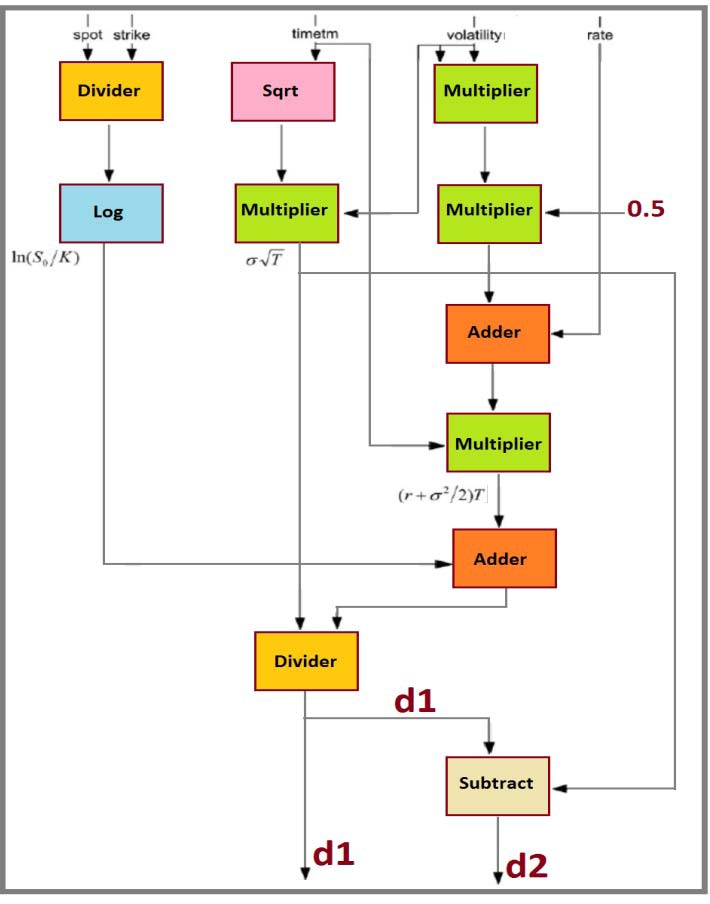
B. D1D2 Block Implementation and Design
The module D1D2 has 5 inputs according to the Eqs. (2) and (3) namely strike price of the option, spot price of the option, risk free interest rate, expiration time, and the market volatility [7]. It takes these inputs and returns the results for the Eqs. (2) and (3).
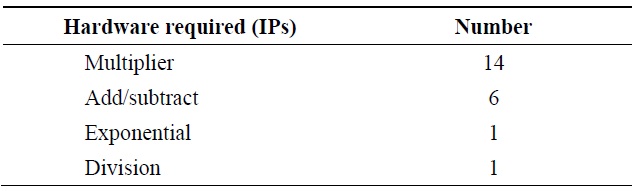
[Table 2.] Resource utilization for D1D2
Resource utilization for D1D2
The resources required for implementation of module D1D2 according to the equations mentioned above are shown in Table 2, and architecture and design flow is show in Fig. 2.
>
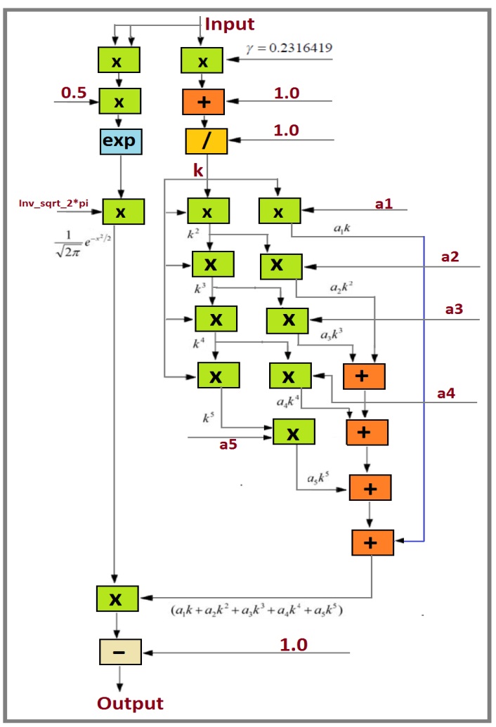
C. CDF Block Implementation and Design
This module has one input and it takes the outputs of D1 and D2. The two outputs are fed into 2 CDF modules, and this is done in parallel to make the design faster. The outcome of the module is CDF for D1 and D2, i.e.,
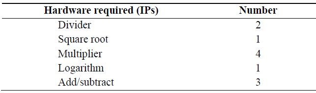
The resources used for the implementation of this module are shown in the Table 3, and the architecture is shown in the Fig. 3.
[Table 3.] Resource utilization for cumulative distribution function
Resource utilization for cumulative distribution function
>
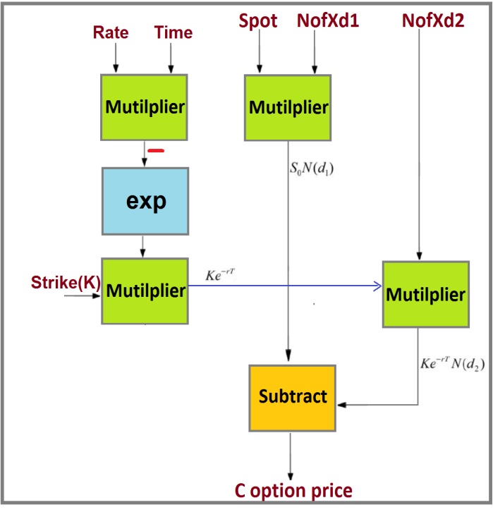
D. Option Price Block Implementation and Design
For computation for European call option price, the inputs rate and time were passed through a multiplier, the then along with minus sign they were passed through exponential and we got result as
The model was tested before proceeding with the Verilog Coding. The design was tested by developing MATLAB and C/C++ models.
In the MATLAB model, first the Eq. (2) (mentioned in chapter-4) which for computation of d1 is implemented followed by the Eq. (3) for d2 and then the results are given to the 2nd block that is the CDF block. In the CDF block the standard normal distribution as described in Eq. (4) is found and the results are utilized to find the CDF.
Lastly, all the results along with the other parameters are given to the last block that is the option price and final result for the call option system is calibrated.
[Table 4.] Resource utilization for complete design
Resource utilization for complete design
The C/C++ verification model [7] was divided into 3 methods namely:
This method is developed using the Eqs. (2) and (3). It takes 5 inputs namely strike price of the option, spot price of the option, risk free interest rate, expiration time, and the market volatility. It takes these inputs and returns the results for the Eqs. (2) and (3).
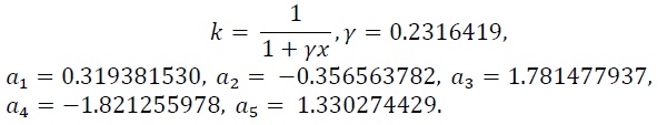
This method is based on the Eqs. (4) and (5). The method take one input at a time and they are the results of D1 and D2, it finds the value of the standard normal distribution function defined in the Eq. (4) (the value for the inverse square root for 2 multiplied by pie that
is 0.39894228040143270286) and the result are the fed into Eq. (5) and finally the cumulative normal distribution function is obtained [7].
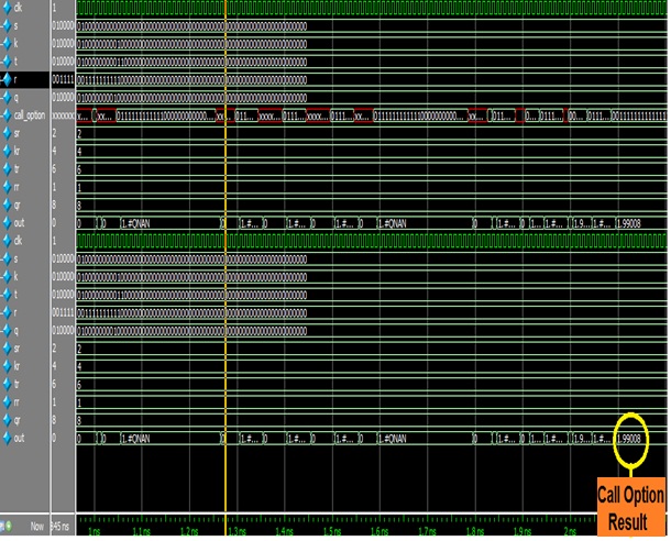
The 3rd and final method computes the value of the European call option, it calls both the previous methods and we finally get the result for of the call option price [7].
>
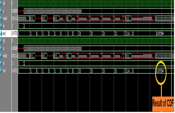
A. Simulation and Synthesis Results
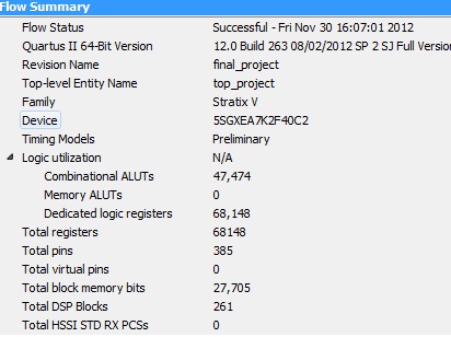
The design was successfully run on Stratix-V FPGA (5SGXEA7K2F40C2) with a frequency of 179 MHz. It performs 180 million transactions per second with initial latency of 208 clock cycles
The simulation results for the modules D1D2, CDF, and call option are show in the Figs. 5?7.
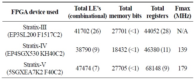
The synthesis results of the complete design are shown in Fig. 8. The resource utilization of complete design for various Altera FPGA families is shown in the Table 5.
[Table 5.] Resource utilization chart of Black Scholes model for various Altera FPGA families

Resource utilization chart of Black Scholes model for various Altera FPGA families
It can be observed from the above table that the design failed on Stratix-III FPGA because it lacked resources. The speed offered by the Stratix-IV FPGA was less as compared to Stratix-V FPGA, so we used the Stratix-V for the successful implementation of the design and maximum frequency achieved was 179 MHz.
In this paper, we implemented a high-performance Black Scholes system on Altera Stratix-V FPGA. It computes the real-time call price for European style option. With the continuous advancements in field of FPGA, it is now easy to implement high performance financial trading applications with high precision, thereby, providing the advantage of improving the performance of the system by implementing complex computations efficiently. We compared Black Scholes system with the models which have been implemented in past, and it was concluded that Black Scholes model provides high performance in terms of speed and accuracy.
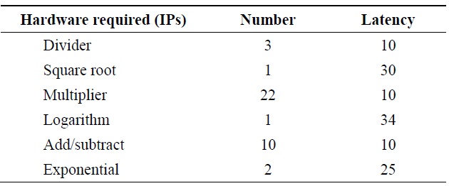
The design estimates real-time call price for European style option at risk free interest rate, and performs 180 million transactions per second with the initial latency of 208 clock cycles. The design runs at a speed of 179 MHz. The design used 3 dividers, 1 square root, 22 multipliers, 1 logarithm, 10 add/subtract, and 1 exponential IPs. The design utilized 68148 logic elements, 27705 memory bits, and 261 total DSP blocks on Stratix-V (5SGXEA7K2F40C2) FPGA.

![Black Scholes and Binomial pricing model comparison [4]](http://oak.go.kr/repository/journal/12437/E1ICAW_2013_v11n3_190_t001.jpg)
![Black Scholes system architecture [7].](http://oak.go.kr/repository/journal/12437/E1ICAW_2013_v11n3_190_f001.jpg)

![Architecture of D1 and D2 [7].](http://oak.go.kr/repository/journal/12437/E1ICAW_2013_v11n3_190_f002.jpg)
![Architecture of cumulative distribution function [7].](http://oak.go.kr/repository/journal/12437/E1ICAW_2013_v11n3_190_f003.jpg)

![Architecture of Call Option price [7].](http://oak.go.kr/repository/journal/12437/E1ICAW_2013_v11n3_190_f004.jpg)