The present paper deals with the problems of yaw angle effects on podded propulsor performance. The study aims at providing insights on characteristics of podded propulsors in azimuthing condition. In this regard, a wide numerical simulation that concerned yaw angle effect measurement on podded propeller performance was performed. The Reynolds-Averaged Navier Stokes (RANS) based solver is used in order to study the variations of hydrodynamic characteristics of podded propulsor at various angles. At first, the propeller is analyzed in open water condition in absence of pod and strut. Next flow around pod and strut are simulated without effect of propellers. Finally, the whole unit is studied in zero yaw angle and azimuthing condition. Structured and unstructured mesh techniques are used for single propeller and podded propulsor. The performance curves of the propeller obtained by numerical method are compared and verified by the experimental results. The characteristic parameters including the torque and thrust of the propeller, the axial force and side force of unit are presented as function of velocity advance ratio and yaw angle. The results shows that the propeller thrust, torque and podded unit forces in azimuthing condition depend on velocity advance ratio and yaw angle.
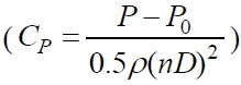
CP Pressure coefficient
D Propeller diameter
Fx Axial force
Fy Side force
J Velocity advance ratio
k Turbulence kinetic energy
KQ Propeller torque coefficient
KT Propeller thrust coefficient
Kfx Axial force coefficient
Kfy Side force coefficient
n Propeller angular velocity (RPS)
P Static pressure
Q Propeller torque
Tpro Propeller thrust
Tpod Pod thrust
Tstrut Strut thrust
Tunit Unit thrust
V Axial velocity

Velocity vector
δij Keronecker delta
ηpro Propeller efficiency
ηunit Total unit efficiency
μ Molecular viscosity
ρ Fluid density
ω Turbulent dissipation rate
ψ Yaw angle

Stress tensor
Recently, podded propulsion systems are widely used in marine industry and becoming more popular, not only for passenger ships, but also for offshore drilling units and naval vessels. The main components of podded propulsor are strut, pod and propeller. In this system, an electrical motor is located inside a steerable pod housing which drives a fixed pitch propeller. The total unit is hung below the stern of ship by strut and can be rotating through 360
Two main configurations of podded systems are puller and pusher types. In the puller type, the propeller is located in the forward face of the pod and upstream of the strut. In the pusher type, the propeller is located in the downward face of the pod and downstream of the strut. Pusher type propellers have lower efficiency than puller type. In pusher type, the propeller works in the wake of the strut. In general, the efficiency of podded propulsor is lower than open water propeller. This matter is due to resistance of pod and strut. Therefore the resistance of unit is an important factor that cannot be ignored.
The conventional propulsion systems such as propeller-rudder systems operate in the hull’s wake flow. Due to the hull’s presence, the flow distribution into the propeller is non-uniform and unsteady. The most significant hydrodynamic advantage of the podded propulsor is that the propeller is set in a more regular flow and works mainly in an open water flow that is uniform which results in little or no cavitation. It is necessary to utilize this system for ship propulsor, especially for vessels which need to be prevented from cavitation (Ghassemi and Ghadimi, 2008).
More recently, due to the market needs and in order to gain more efficiency by the podded systems, marine researchers have rigorously pursued this topic and much effort has been devoted to explore it numerically and experimentally. During the past two years, the 1st and 2nd T-Pod conferences have been held at the University of Newcastle (UK) and Universite de Bretagne Occidentale Brest (France) in 2004 and 2006 (ITTC, 2005; ITTC, 2008), respectively, and many researchers (like Kinnas, 2006; Bal et al., 2006) presented their latest findings. One of main operational problems of podded systems is bearing failure (Carlton, 2008). This mechanical failure occurs when there are unpredicted forces and moments which act on the podded system especially in yaw angle. Therefore, the study on variation of forces and moments in azimuthing condition is very important and required for design and optimization of podded systems.
Experimental studies of Szantyr (2001) were one of the early works for podded propulsor in azimuthing condition. He measured axial and transverse force and moment for podded drive to ±15° yaw angle. Reichel (2007) also presented result of comprehensive maneuvering open- water tests of a pusher drive. Steering forces were measured in the range of yaw angle from -45° to +45°. In the recent work, Amini and Steen (2011) reported systematic model test results of the podded drives in different velocity advance ratios and different yaw angles. The tests were performed on the pulling and pushing modes for both open water and in behind conditions. An important study of this problem is the work carried out by Islam et al. (2007). Particular test equipment was designed and several different measurements were considered. The podded propulsor was tested in puller and pusher condition in different yawing angle from -30° to +30°. Their results showed that the unit force and moment coefficient depend on velocity advance ratio, yaw angle and yaw direction.
Numerical analysis of podded drive in azimuthing condition has not thus far been adequately explored. It is definitely imperative that we use more reliable numerical method in the design of such a propulsion system in order to understanding about flow pattern around podded drives. The present study focuses on hydrodynamic analysis of podded drive in azimuthing condition. The results included are the open-water characteristics of the single propeller and hydrodynamic performance of the puller type of the podded drive at various yaw angles.
It is a common practice to perform a model test to evaluate the hydrodynamic performance of a marine propeller or propulsion system. However, the model test is usually expensive and time-consuming. Computational fluid dynamics (CFD) is a powerful tool for analyzing the performance of ship propulsion systems. Two methods are usually used in this field of CFD: inviscid and viscous methods. The inviscid method is usually based on potential theory, while the viscous method uses numerical solution of the Navier-Stokes and the continuity equations; offering many advantages over potential flow based methods. The viscous method has traditionally been employed for flow problems where turbulence, boundary layer, wake, and viscous resistance are important. Different solution approaches have been proposed during the past few years, such as the direct solution of the Navier-Stokes equations and the solution of Reynolds-Averaged Navier-Stokes (RANS) equation.
In order to study the effect of yaw angle on podded drive performance, different numerical methods have been used from potential method or potential/viscous method to pure viscous method. In azimuthing condition, there is interaction between the pod, propeller, and strut. Therefore, the viscous effect is an important phenomenon in hydrodynamic analysis.
The numerical methods based on potential flow theory have been used widely and successfully to predict the performance of conventional propellers. Ghassemi and Ghadimi (2008) predicted podded drive performance using potential flow method. Also Liu et al. (2009) applied unsteady panel method code for predicting unsteady forces, torques and bending moments for a podded propulsor unit model at various yaw angles. Their results showed that there is a discrepancy between numerical results and experimental data at large yaw angles. Due to viscous effects in large yaw angle, the interaction between propeller, pod and strut increases. Also at these angles drag of propeller, pod, and strut increase to high values because of flow separation. For this matter, potential results should be corrected at large yaw angles by estimating proper value for pod drag.
RANS solvers are capable to take into account the viscous and turbulence effects for podded drive. First RANS simulation for podded drive has been done by Sanchez-Caja et al. (1999). They presented a fully viscous method for analysis of these systems. Also, Koushan and Krasilnikov (2008) used unsteady RANS solver for simulating the flow around pulling and pushing pod propeller in azimuthing condition from -45° and +45° yaw angle.
In this work, the finite volume based RANS solver is applied to predict the hydrodynamic performance of marine propeller and podded propulsor. By these simulations, characteristics of flow around the marine propeller and puller podded drive are presented including pressure distribution and open water performance curves in zero angle and oblique flow. The computational results are discussed and compared with the experimental data.
Resulting unit thrust from podded propulsor is sum of three components:

where Tpro, Tpod, and Tstrut are components of thrust from the propeller, pod, and the strut respectively.
For podded propulsor, coefficients of propeller thrust, unit thrust, axial and side force are defined as:

where Fx and Fy are total forces on the whole unit in x and y direction respectively. These coefficients are important factors in design of podded drives affecting propulsion and maneuvering specifications. Also velocity advance ratio, propeller efficiency, and total unit efficiency can be defined as:

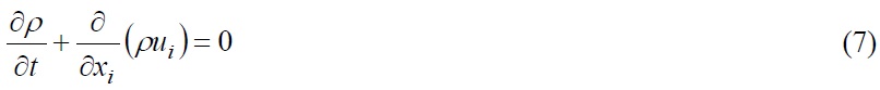
The governing equations for the mass and momentum conservation can be stated as:


where
denotes the velocity vector, p is the static pressure and
represents the stress tensor given by:
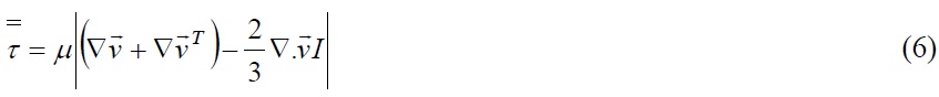
In which

where
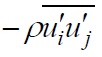
shows the Reynolds stresses.
It is rather difficult to model the components of Reynolds stress tensor, because it requires detailed and unavailable data about turbulent structures in the flow. The k-ε and k-ω models are the most widely used turbulence models for external aerodynamics and hydrodynamics analyses. In this paper, the two equation standard k-ω model which was developed by Wilcox (1998) is employed where one equation involves the turbulence kinetic energy (k) representing the velocity scale and the other takes the turbulent dissipation rate (ω) into account representing the length scale. The two-equation standard k-ω turbulence model accounting for the effect of turbulence is


where σk and σω are the turbulent Prandtl numbers for k and ω, respectively. The turbulent viscosity, μt, is computed by combining k and ω as follows:

The rotation of the propeller in the fluid environment is modeled using Moving Reference Frame (MRF) method. By using MRF method, the flow around propeller can be modeled in a steady-state manner. In this case, governing equations is solved with additional acceleration terms. The computational domain is divided into stationary and moving frames. For an arbitrary point in solution field, the absolute velocity,
can be defined with the following relation:

where

is position vector from the origin of the moving frame and

is the angular velocity vector.
The governing equations of fluid flow in a moving reference frame can be written in two different ways: absolute velocity formulation or relative velocity formulation. The mass and momentum equations in the relative velocity formulation can be stated as:

where
is the Coriolis acceleration and
is the centripetal acceleration.
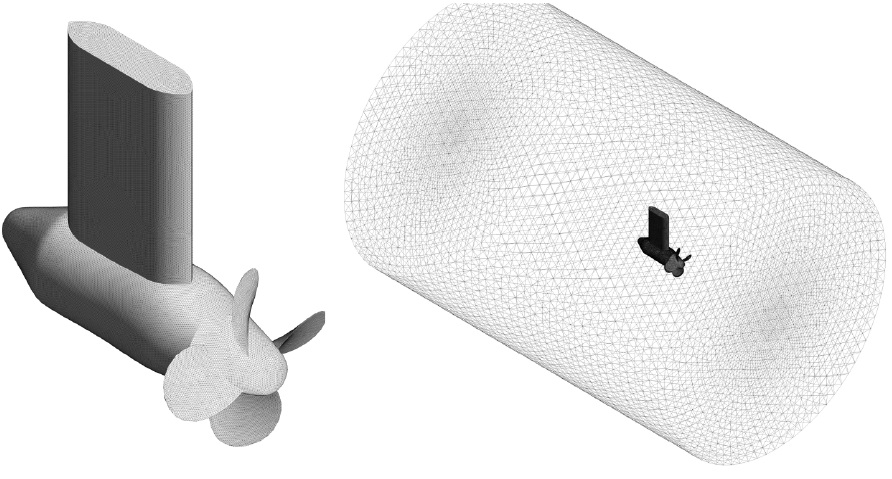
For better understanding of the behavior of forces and moments act on podded drives, three models were created: a single propeller model, pod and strut alone model and a puller podded drive. The Cartesian coordinates are used, where (
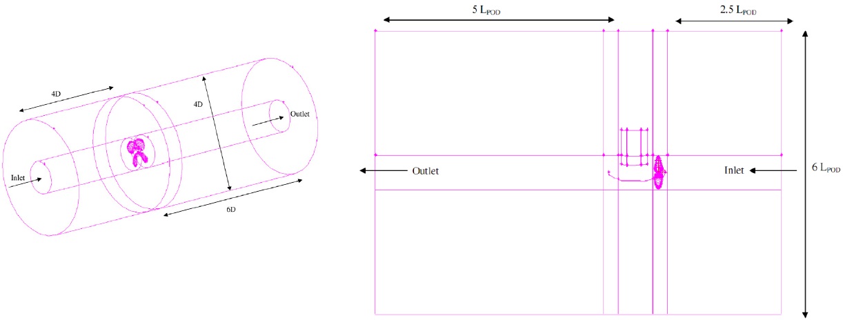
In order to model the propeller in the fluid environment the solution field is divided into global and sub-domain cylindrical frames, as depicted in Fig. 1. The sub-domain frame simulates the propeller rotation and employs the Coriolis acceleration terms in the governing equations for the fluid. The global frame surrounds the sub-domain frame. The global frame is a circular cylinder with 4
For a single propeller, the solution field is divided into six blocks. Rotating block is meshed with unstructured tetrahedral cells and the other blocks are meshed with structured hexahedral cells. The unstructured grid causes a smoother discretization near the leading and trailing edge of the propeller. Surface of propeller and hub are meshed with the size of 0.01
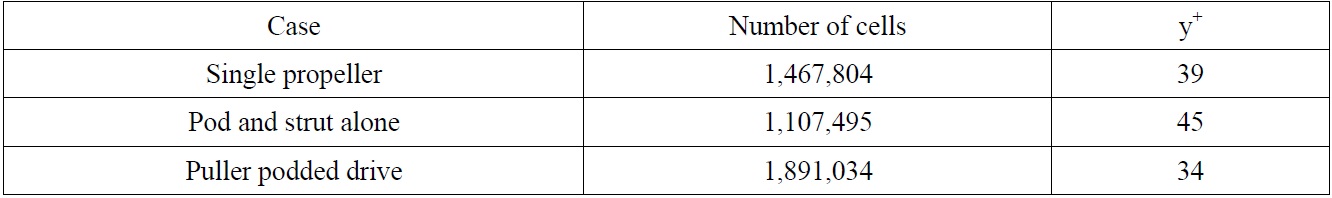
[Table 1] Grid sizes and y+ values.

Grid sizes and y+ values.
BOUNDARY CONDITIONS AND NUMERICAL SETUP
The governing equations of this problem are solved by the finite volume method based on the RANS equations. The Fluent 6.3 software was used to solve the RANS equations. Based on literatures published in the application of Fluent in the simulation of the flow around conventional propellers (Seo et al., 2010; Kulczyk et al., 2007), it is used in this study to investigate the open water hydrodynamic performance of the podded propeller.
The simple algorithm is used for solving the pressure-velocity coupling equations. The second order upwind discretization scheme is utilized for the momentum, turbulent kinetic energy, and turbulent dissipation rate in this problem.
The fluid (water) was assumed as an incompressible fluid, therefore; on the inlet boundary uniform velocity was imposed and on the outlet boundary, the static pressure was set to zero. The no-slip wall condition was imposed on the propeller blades, pod, and strut.
The numerical method mentioned above is employed for the simulation of viscous flow around conventional marine propellers and puller podded drive. At first, the propeller is analyzed in open water condition in the absence of the pod and strut. Next flow around pod and strut are simulated without effect of propellers. Finally, the whole unit is studied in zero yaw angle and azimuthing condition.
In this section, a single propeller model is selected. This is base propeller model geometry with -15° hub taper angle that was used by Liu in podded propeller research program (Liu, 2006). The characteristic curves and performance data of the propeller are determined by the experimental tests in the cavitation tunnel. Tables 2 and 3 give the main dimensions and particular geometry data for propeller model respectively.
In order to get an evaluation of the grid uncertainty, the grid dependency study is conducted for single propeller. The study of the propeller performance in the open water condition was carried out for three different mesh resolutions. The best compromise between element size and accuracy has been obtained by results of this work. These models were simulated at
[Table 2] Main dimensions of propeller model.
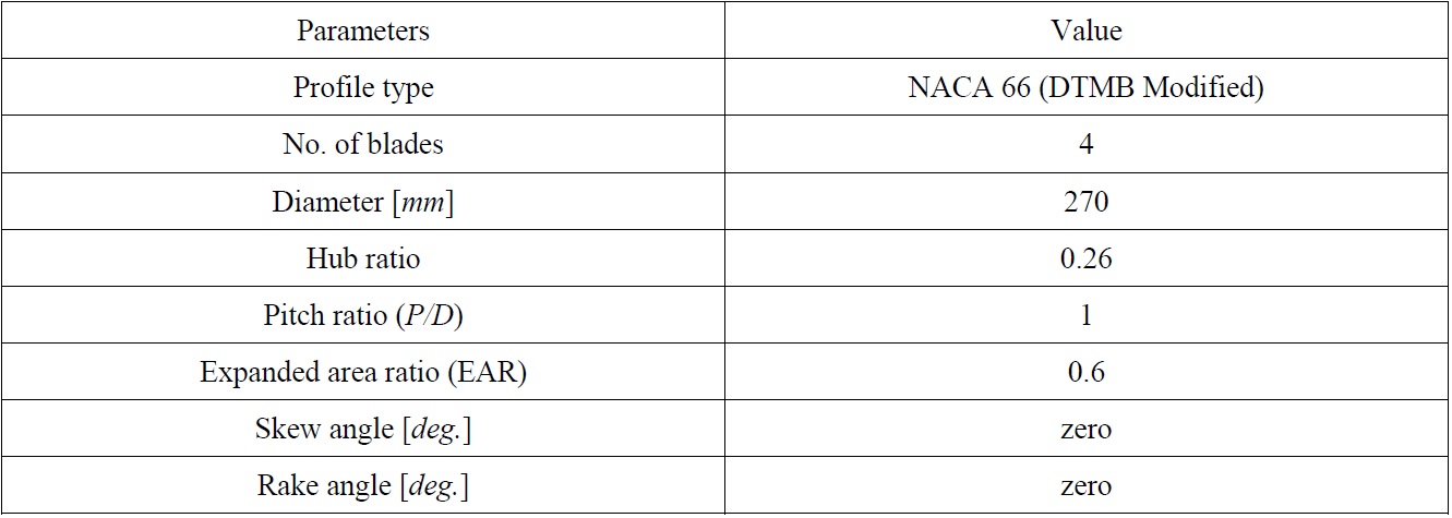
Main dimensions of propeller model.
[Table 3] Particular of propeller geometry.
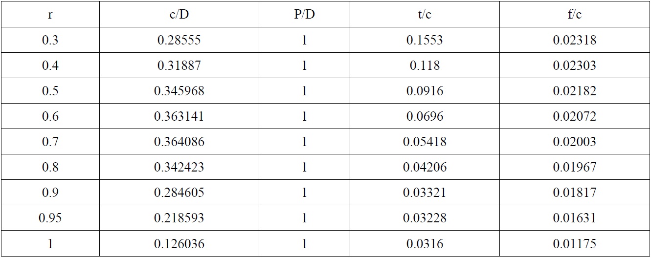
Particular of propeller geometry.
The relative error of CFD results with respect to the experiments for grid dependency study.
Assuming the constant rotational velocity for the propeller, its performance is investigated for different inlet velocities to obtain the characteristics of the propellers in open water conditions. The propeller angular speed is 15
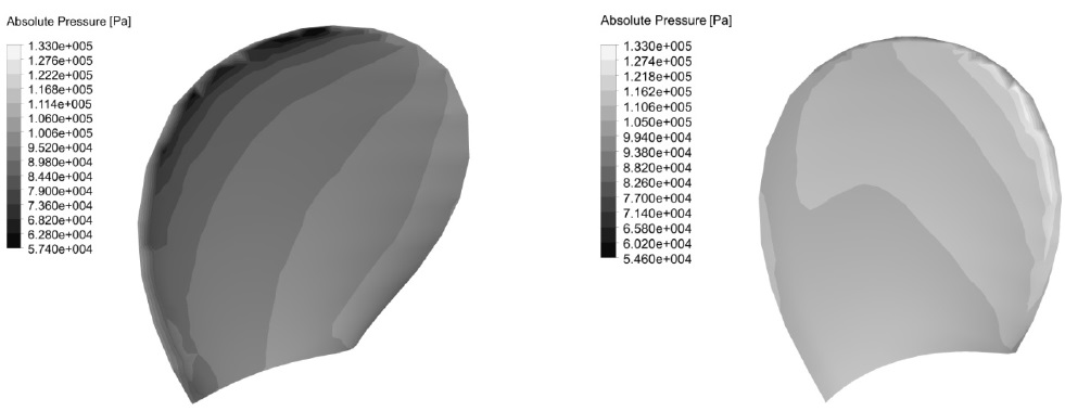
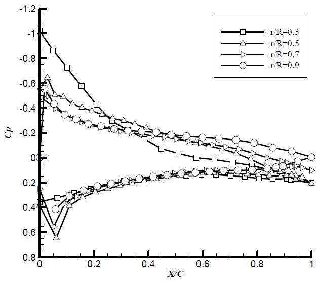
Fig. 3 represents the pressure distribution on back side and face side of the propeller at
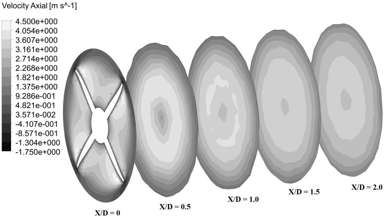
Also, the axial velocity distribution for propeller in transverse planes is shown in Fig. 5. It is clearly observed that the velocity at the propeller downstream position is high. In
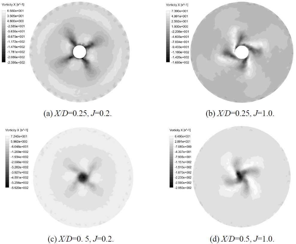
at four radii (
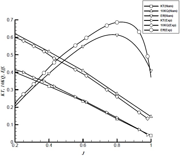
Fig. 7 shows the hydrodynamic characteristic curves obtained by analysis and its comparison with the experimental data. The results show that there is a good agreement between the experimental data and CFD results particularly for advance ratio 0.2 to 0.8. It can be seen that propeller thrust coefficient is underpredicted, while the propeller torque coefficient is overpredicted. In these range of advance ratio (
[Table 5] The relative error of CFD results with respect to the experiments for single propeller.

The relative error of CFD results with respect to the experiments for single propeller.
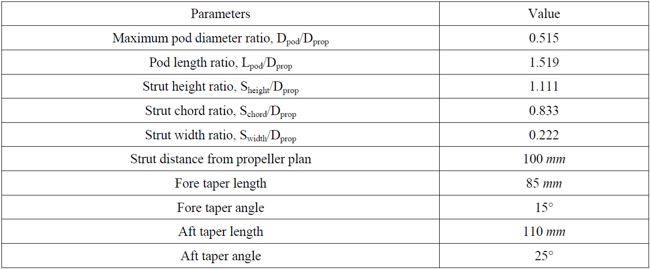
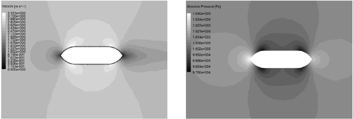
The flow around the pod and strut is fully 3-dimensional and non-symmetric in nature. In this section, the pod and strut have been analyzed in RANS solver without propeller effects. The non-dimensional data of the pod and strut is presented in Table 6. Profiles of the pod and strut is similar to the one used by Islam et al. (2007). A cylindrical domain was created around the pod and strut and an unstructured mesh was used. The no-slip wall boundary conditions are applied on the pod and strut body. Flow characteristics around the pod and strut were evaluated in zero yaw angle and azimuthing condition at different inlet velocity. Yawing angles of the pod and strut are changed from +30° to -30° with 5° increment. The inflow velocity is selected same as single propeller advance ratio from 0.2 to 1.0.
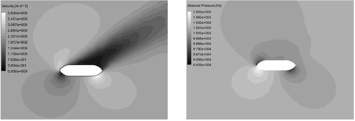
Figs. 8 and 9 show velocity and pressure distribution predicted on the strut at zero and +30 yaw angle respectively. These counters are plotted in
[Table 6] The non-dimensional main particulars of pod and strut.

The non-dimensional main particulars of pod and strut.
This section presents a validation study of RANS predictions of podded drive in azimuthing condition. A model of puller podded drive including propeller, pod, and strut has been established and the whole of unit has been analyzed in RANS solver. Flow characteristics around the propeller, pod and strut were evaluated. The puller drive is studied in zero yaw angle and azimuthing condition. Computational results are compared with experimental works of Islam et al. (2007). The total forces on puller drive in each direction and propeller thrust and torque are computed for a range of advance ratios from 0.2 to 0.8. In these calculations, the angular speed of propeller is set to 15
[Table 7] The relative error of CFD results with respect to the experiments for puller drive.

The relative error of CFD results with respect to the experiments for puller drive.
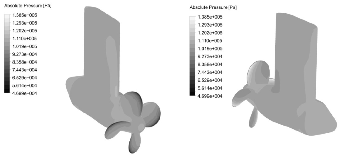
Fig. 10 shows pressure distribution on pod, strut, and propeller at zero yaw angle at an advance ratio of
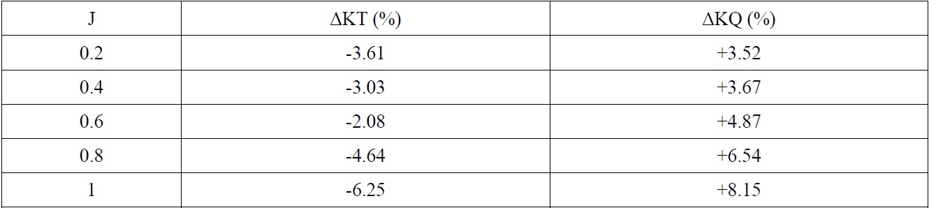
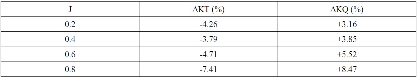
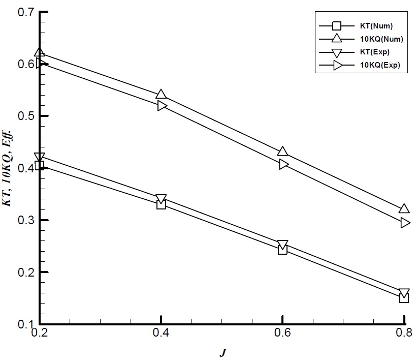
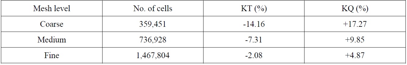
The propeller thrust and torque coefficients for puller podded drive in straight condition are presented in Fig. 11 and compared by the experimental results. There is a good agreement between the numerical and the experimental results. The relative error of CFD results with respect to the experiments are shown in Table 7. It can be seen that the relative error of KT and KQ is less than -5% and +6% within the range
Also, the performance of the puller podded drive is studied in azimuthing condition and results are compared by the experimental data. The results included are the propeller thrust coefficient, propeller torque coefficient, total unit axial force coefficient, and total unit side force coefficient at various yaw angles.
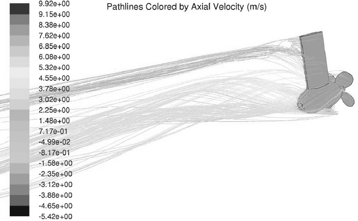
The streamlines at downstream of the puller drive for -30° yaw angle at an advance ratio of
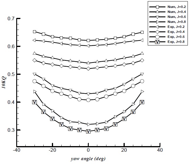
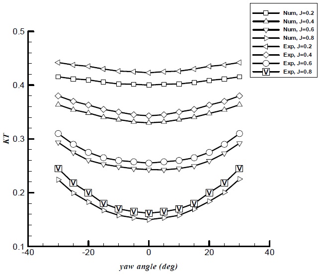
Figs. 13 and 14 show the propeller thrust and torque coefficients for a range of advance ratios and yaw angles. According to these results, the propeller thrust and torque predictions for all advance ratios are in overall agreement with the test data. In general, the relative error for propeller torque is greater than that for propeller thrust at the same velocity advance ratio. Also, larger deviations are seen at high heading angles. The results for
Fig. 13 shows the propeller thrust coefficient for a range of advance ratios and yaw angles. In positive angles and negative angles, the propeller thrust coefficient increases with increasing yaw angle. This behavior is similar for all advance coefficients. As seen in Fig. 13, curves of the propeller thrust coefficients are symmetrical at positive and negative yaw angles. In azimuthing condition, the effective advance coefficient in the direction of the propeller axis is reduced. This results in higher thrust in the corresponding operating conditions.
The variation propeller torque coefficients are shown in Fig. 14. The same behavior is found in the propeller torque coefficient. The propeller torque coefficient increases when yaw angle is increased from zero to positive or negative yaw angles and the propeller thrust coefficients are approximately symmetrical at positive and negative yaw angles.
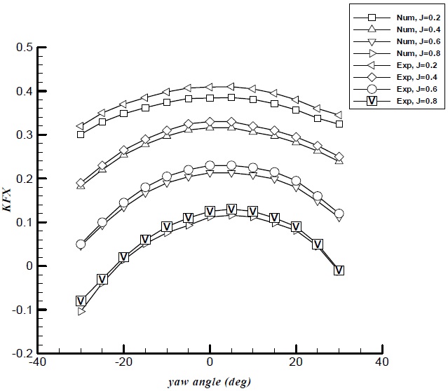
The total unit axial and side force coefficients for the puller podded drive at different yaw angles are presented in Figs. 15 and 16 and compared with test data. In general, the total axial and side forces are predicted close to the test data.
As shown in Fig. 15, the total unit axial force coefficient decreases with increasing yaw angle. Curves of the axial force coefficients are not symmetrical at positive and negative yaw angles. In puller podded drive, the inflow on the pod and strut is influenced by propeller induced wake flow and the interaction between the propeller wake and the strut is dominated. This results in asymmetry in total unit axial force curve. For all advance ratios, the maximum value of the axial force coefficient is obtained at yaw angle +5° approximately.
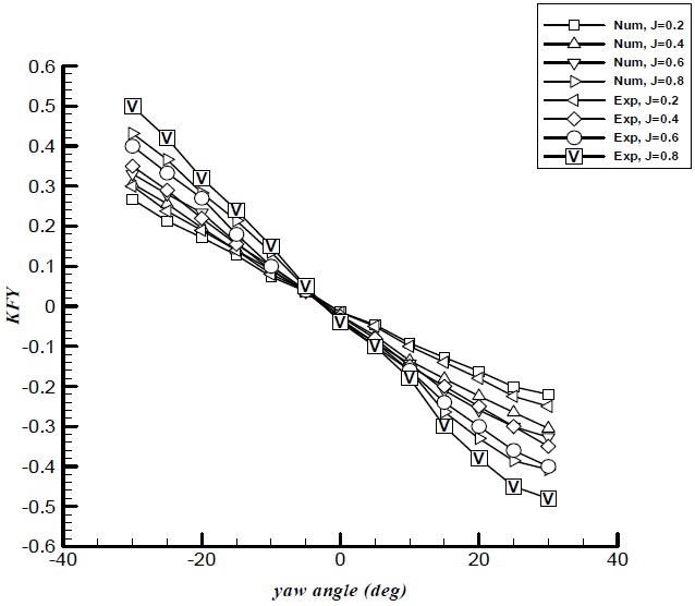
Fig. 16 shows the side force coefficient variation with yaw angle. As shown, for all advance coefficients, the side force coefficient increases when yaw angle is increased to the left (negative yaw angle) or right (positive yaw angle). Also, side force coefficients for puller drive increase with increasing advance coefficient. The zero side force is found at the small yaw angle about -2°. Due to the propeller wake rotation and strut interactions, there is a small side force in straight condition (zero yaw angle) for podded drives.
In this paper, a finite volume based RANS solver has been used to evaluate the performance of the podded drive in straight and azimuthing condition. The rotation of the propeller was modeled using MRF method and k-ω model was selected as turbulence model. Hydrodynamic analysis of a single propeller, pod and strut alone, and puller drive was investigated at various yaw angles and operating conditions. Open-water characteristics of the propeller and puller podded drive axial and lateral forces were compared with the experimental data.
Based on the result of CFD simulation, Open-water characteristics of the single propeller are in good agreement with the experimental data. Also the RANS predictions of puller drive forces for all advance ratios are in overall agreement with the test data. The relative error for propeller torque is greater than that for propeller thrust at the same advance ratio and larger deviations are seen at high yaw angles. In general, the thrust, torque, and unit force coefficients showed a strong dependence on the velocity advance ratio and yaw angle.
The numerical investigation of the flow characteristics around the puller podded drive at different yaw angles showed that for all advance coefficients, the propeller thrust coefficient increases with increasing yaw angle. This behavior is similar for negative angles and positive angles, and curves of the propeller thrust coefficients are symmetrical at positive and negative yaw angles. The same behavior is found in the propeller torque coefficient. At azimuthing condition when yaw angle is changed from straight condition to positive or negative angle, the effective velocity advance coefficient in the direction of the propeller axis is reduced. This results in higher thrust in the corresponding operating conditions.
Besides, the study proved that the total unit axial force coefficient decreases with increasing yaw angle and curves of the axial force coefficients are not symmetrical at positive and negative yaw angles. Induced velocities from propeller change the inflow to the strut and pod. At large yaw angles, as the flow passes over the propeller, the oblique flow and propeller slipstream induce strong vortex and separation on the pod and strut. Therefore the surface pressure contours of the pod and strut are asymmetrical and results in asymmetry in total unit axial force curve.
The results also indicated side force coefficients increases with increasing yaw angle and velocity advance ratio. In puller podded drive, due to the propeller wake rotation and strut interactions, there is a small side force in straight condition.