Cross-shore sediment transport is very important factor in the design of coastal structures, and the beach profile is mainly affected by a number of parameters, such as wave height and period, beach slope, and the material properties of the bed. In this study cross-shore sediment movement was investigated using a physical model and various offshore bar geometric parameters were determined by the resultant erosion profile. The experiments on cross- shore sediment transport carried out in a laboratory wave channel for initial base slopes of 1/8, 1/10 and 1/15. Using the regular waves with different deep-water wave steepness generated by a pedal-type wave generator, the geometrical of sediment transport rate and considerable characteristics of beach profiles under storm conditions and bar parameters affecting on-off shore sediment transport are investigated for the beach materials with the medium diameter of d50=0.25, 0.32, 0.45, 0.62 and 0.80 mm. Non-dimensional equations were obtained by using linear and non-linear regression methods through the experimental data and were compared with previously developed equations in the literature. The results have shown that the experimental data fitted well to the proposed equations with respect to the previously developed equations.
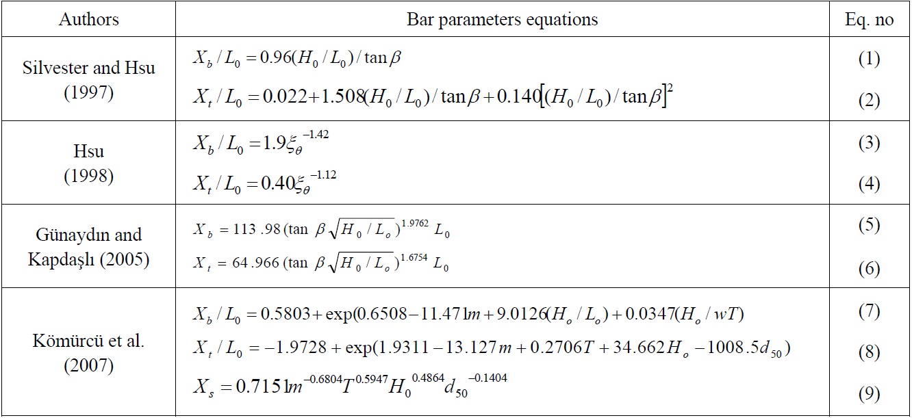
Most problems of coastal engineering are dependent on a number of parameters. There are lots of parameters affect design of coastal structures such as the wave height and period, the beach slope and the properties of the bed. Bar parameters caused by cross-shore sediment transport are very important for design of coastal structures. Various parameters such as wave conditions, bed slope, and characteristics of sediment particles affect the cross-shore sediment transport discharge and consequently the coastal profiles. There are many theoretical and experimental studies which carried out by researchers. Previously studies in this subject are summarized as follows. Cross-shore sediment transport and on coastal features consequential of diverse factors were studied by (Saville, 1957; Dean, 1973; Noda, 1972; Gourlay, 1980; Sawaragi and Deguchi, 1980). Beach profiles were classified such as by Johnson (1949), Iwagaki and Noda (1962), Nayak (1970) and Hattori and Kawamata (1980). A model was offered to describe onshore-offshore sand transport in the surf zone by Sunamura and Horikawa (1974). The model was based on the physical consideration that the net transport attains a state of equilibrium. They proposed beach classification based on displacement of topography from the initial beach slope. Using these parameters, the direction of onshore-offshore transport and the beach profile in the surf zone were expressed. Larson and Kraus (1989) studied erosion and deposition profiles and proposed a formula for bar parameters using experimental data as well as for erosion and deposition criteria. Silvester and Hsu (1997) determined beach profile parameters by non-linear regression techniques using various experimental data obtained from previous works. In this study, the proposed formula for bar parameters is given in Table 1. Watanabe et al. (1980) developed a three-dimensional numerical model to estimate cross-shore sediment transport. Larson (1996) produced a numerical model to compute cross-shore sediment transport and the beach profile under effects of regular waves and in this modeling, three cases of variation of profiles were studied. This model enables the investigation of bar-forming erosion in equilibrium, berm erosion and effects of broken waves on offshore bar; this model is well fitted for erosion conditions, but not for deposition conditions. Experimental and theoretical works carried out by Hsu (1998). He determined the geometry of offshore bar. He concluded that cross-shore waves traveling with variable angles make the beach profile be in equilibrium. Obtained equations for bar parameters are also given in Table 1. Ruessink et al. (2002) have made an attempt to determine long time variation of bar crest near beach profile using the remote sensing method. Gunaydın and Kabda?lı (2003) carried out experiments by studying the characteristics of coastal erosion using a model in which the mean diameter of particles and the beach slope are 0.35
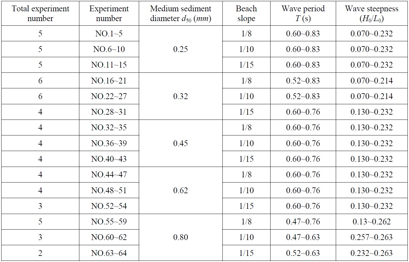
In this study, experiments were carried out on cross-shore sediment transport in order to investigate the affecting bar parameters on-off shore sediment transport for five different beach materials of mean grain diameter d50 equal to 0.25, 0.32, 0.45, 0.62 and 0.80
[Table 1] Currently used equations for determination of bar parameters.

Currently used equations for determination of bar parameters.
Under the storm conditions, experiments were carried out in a wave channel of 12
[Table 2] Experimental conditions and bar parameters.
Experimental conditions and bar parameters.
In order to investigate the sediment movement which occurs after the storm conditions and the resultant geometrical features of the beach profiles, the experimental conditions were arranged according to the parameter C (it would be greater than 8).
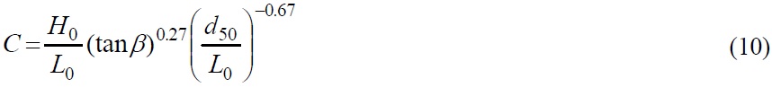
where C is profile parameter, H0 is deep water wave height, L0 is deep water wave length, tan
C < 4 ................ accretion-summer profile
4 < C < 8 .......... equilibrium profile
8 < C ................ erosion-winter profile
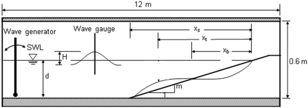
In the current study, cross-shore sediment transport and bar parameters under the storm conditions were investigated. The beach profiles which came out in different sediment diameters, coast slopes and bar parameters affecting the formation of profiles were investigated. Bar parameters which occurs as results of the beach erosion are investigated and given in Fig. 1. In the Fig. 1, Xb is horizontal distance between the initial bar point and original shoreline, Xt is horizontal distance between the bar crest and original shoreline, Xs is horizontal distance between the final bar point and the original shoreline, H is the wave height, d is the water depth, still-water level (SWL).
>
Analysis method of experimental results
Experimental results were examined using linear and non-linear regression methods to obtain equations defining the bar parameters. Two equation types were determined in regression analyses, power (PF) and linear (LF). These functions are given respectively as follows:


Experimental results were examined in detail and used to obtain the fittest equations containing bar parameters using nonlinear regression method. Different regression analyses were applied on bar parameters.
>
Dimensional and non-dimensional variables
Experimental results were made non-dimensional to minimize measurement errors due to laboratory conditions. In this study, non-dimensional bar parameters were used for estimation process. Xb, Xt and Xs considered as an independent variable and was obtained from dividing by
In this study, bar parameters occurred by winter profiles under storm conditions were investigated. As a result of experimental study, bar parameters for each experiment were calculated. Regression analysis was implemented and non-dimensional equations were presented. Non-dimensional regression analysis was applied using results obtained from 64 experiments for Xb, Xt and Xs . The determination coefficient for non-dimensional dependent and independent variable alternatives were computed by non-dimensional regression techniques using various function types.
The dimensionless dependent variables were used as
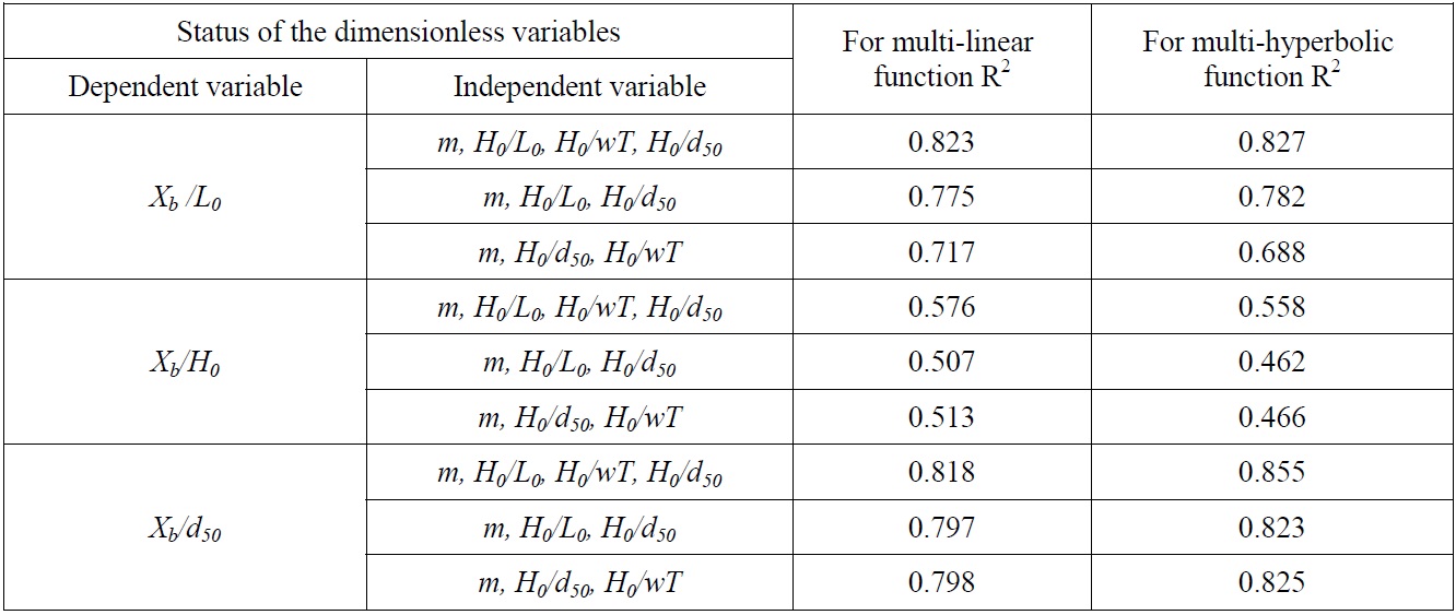
[Table 3] Determination coefficients for dimensionless alternatives variables for Xb.

Determination coefficients for dimensionless alternatives variables for Xb.
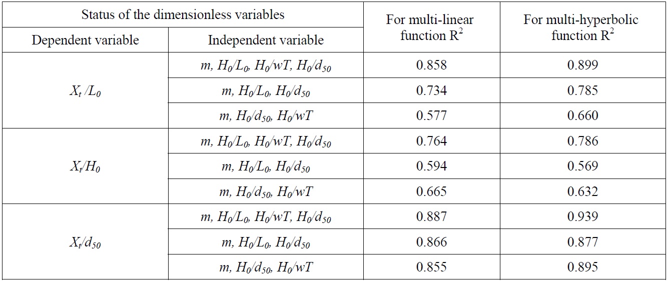
[Table 4] Determination coefficients for dimensionless alternatives variables for Xt.

Determination coefficients for dimensionless alternatives variables for Xt.
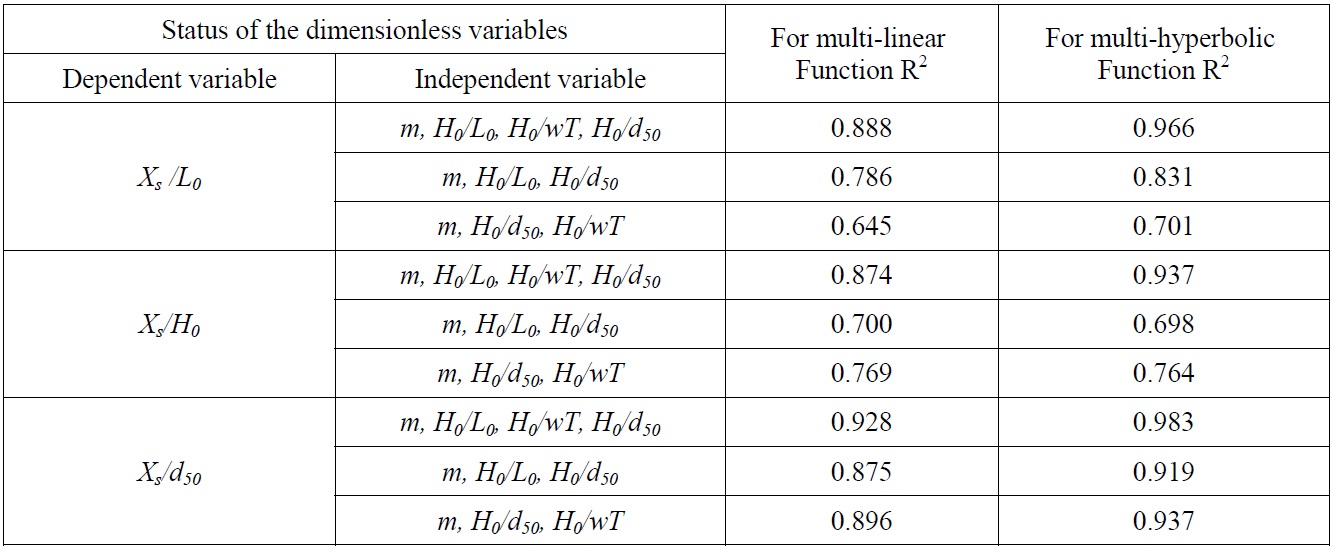
[Table 5] Determination coefficients for dimensionless alternatives variables for Xs.

Determination coefficients for dimensionless alternatives variables for Xs.
[Table 6] Regression coefficients obtained from dimensionless regression analysis for Xb.

Regression coefficients obtained from dimensionless regression analysis for Xb.
[Table 7] Regression coefficients obtained from dimensionless regression analysis for Xt.
Regression coefficients obtained from dimensionless regression analysis for Xt.
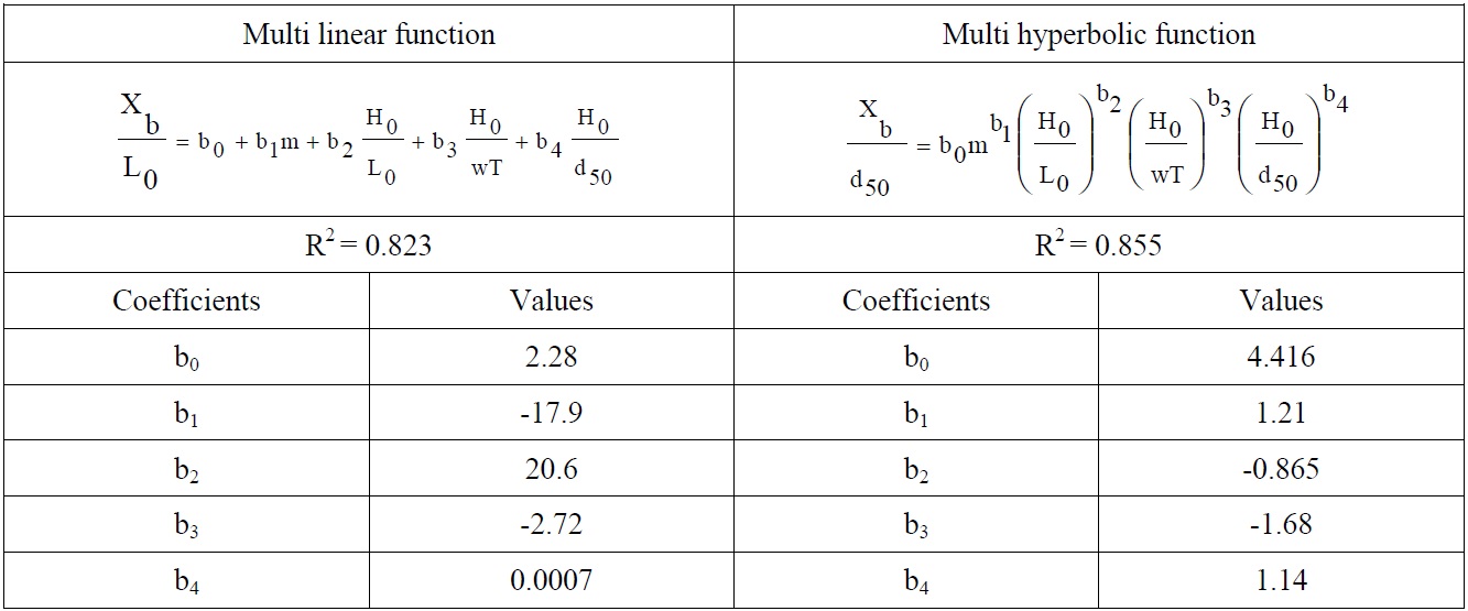
[Table 8] Regression coefficients obtained from dimensionless regression analysis for Xs.
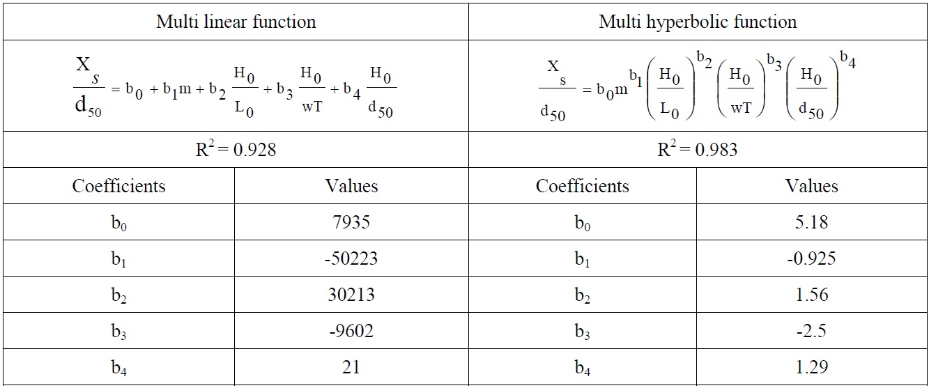
Regression coefficients obtained from dimensionless regression analysis for Xs.
As seen from the Tables 3-5 that, the maximum value of determination coefficient for linear function occurs in the case of
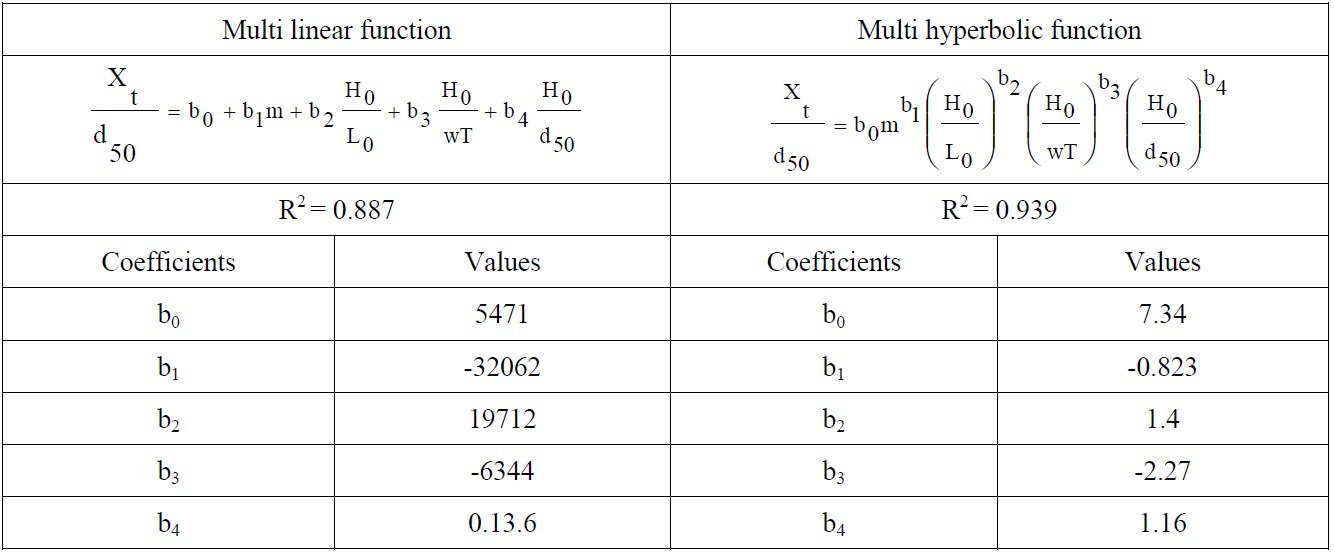
According to the determination coefficient in Tables 6-8, multi hyperbolic functions give better results according to the multi linear functions. The equations derived from the dimensionless hyperbolic functions are presented below for bar parameters.
Proposed Equation for Xb

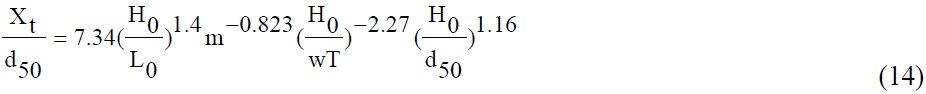
Proposed Equation for Xt
Proposed Equation for Xs

>
Horizontal distance between the initial bar point and original shoreline (Xb)
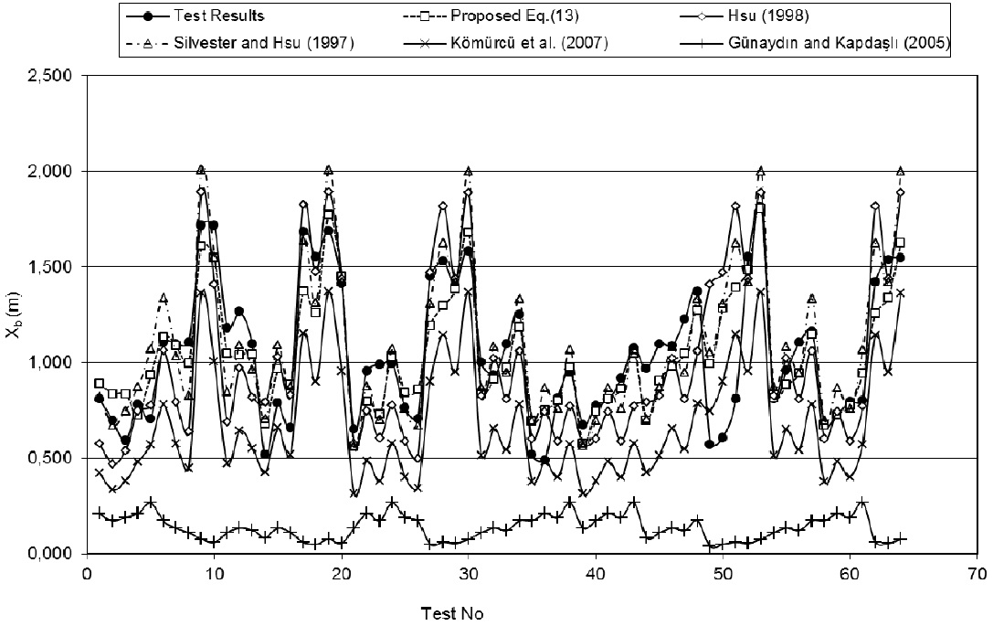
Comparisons of proposed equation (Eq. (13) for Xb and previously developed equations with each other according to the experimental results are shown in Fig. 2. Eq. (13) produces best results which are very close to experimental results as indicated
in Fig. 2. Silvester and Hsu’s equations exhibit similar trends with experimental results despite small deviations with respect to other equations. Results of Hsu’s equation (Eq. (3)) show a good agreement with experimental results in a certain range. Results of Komurcu’s equation (Eq. (7)) are different from Hsu’s equation (Eq. (3)). Gunaydın and Kapdaslı’s equation (Eq. (9)) gives rather different results according to the experimental results and other equations.
>
Horizontal distance between the bar crest and original shoreline (Xt)
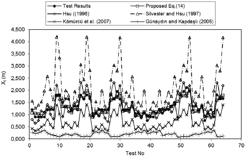
When the proposed equation (Eq. (14)) is compared for horizontal distance between the bar crest and original shoreline (Xt) , Eq. (14) gives best results according to the experimental results. (Fig. 3). Hsu equations (Eq. (4)) produces best result with respect to other equations (Eqs. (2), (6) and (8)) for experimental conditions when compared with each other. Silvester and Hsu’s equation (Eq. (2)) gives also good results according to the experimental results. But Gunaydın and Kapdaslı’s equation Eq. (6) and Komurcu et al.’s equation Eq. (9) shows similar results. Their equations produce different results than the other equations.
>
Horizontal distance between the final bar point and the original shoreline (Xs)
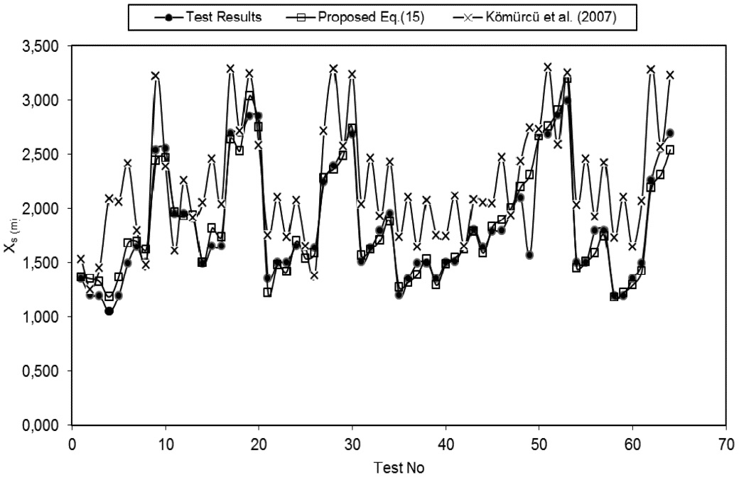
For horizontal distance between the final bar point and the original shoreline (Xs), comparison of best equation (Eq. (15)) and previously developed equations with each other in terms of experimental results are shown in Fig. 4. Considering the equations and the experimental results, a good fit is observed between proposed equation (Eq. (15)) and experimental results. Komurcu et al. equation (Eq. (9)) results are close to the experimental results and proposed equation (Eq. (15)).
In this study, 64 experiments were carried out to determine bar parameters (Xb, Xt, Xs) as functions of H0, T, m and d50, and the results are given in tables. For each bar parameter, nondimensional equations were obtained by applying nonlinear regression methods. The fittest equations for each bar parameter are obtained by comparing these equations with previously developed equations.
According to the regression analysis results, best equations for Xb, Xt, Xs are Eqs. (13), (14) and (15) respectively. The proposed equations are closer to experimental results than those of previously developed equations. For all parameters, Hsu and Silvester and Hsu’s equations give best results according to the experimental results and proposed equations. Gunaydın and Kapdaslı and Komurcu et al. equations doesn’t provide good fit with the other equaitons. It should also be emphasized that a number of experimental data used in this study is greater than those obtained from previous works, hence this helps obtain better results in terms of reliability and reproducibility.