As oil prices have soared recently, great effort to reduce fuel expenses has been made throughout all industries. According to studies that analyzed the effect of route planning for the economic efficiency of ships, fuel expenses account for more than 40% of the operational cost (Journee and Meijers, 1980).
This study was conducted to find ways to determine economical shipping routes that can minimize fuel expenses by considering the sea state. The sea state includes the wave state regarding wave height and wave direction, and the wind state regarding wind speed and wind direction. Economical shipping route determination has been defined previously as “optimal track routing,” “weather routing,” or “optimal ship routing” (Lee and Kim, 2001).
The most representative method for determining an optimum route is the isochrone method proposed by Hanssen and James (1960), which has been used for a long time because it is easy to calculate. Hagiwara (1989) proposed a revised isochrone method, which is easy to calculate with computers. Jung and Rhyu (1999) conducted a study for determining the economical shipping route using the A* algorithm. Choi et al. (2007) and Park et al. (2004) proposed methods that estimate fuel consumption by calculating the reduced amount of the ship’s speed based on a record of sea voyages and weather forecast data, and determined economical shipping routes using an 8-point Dijkstra algorithm. However, these methods do not reflect realtime marine information. In addition, there have been difficulties in finding economical shipping routes in complex maritime areas that have many islands or require considerable memory and time to determine the route. This study proposes a method for determining economical shipping routes after estimating fuel consumption by considering the sea state based on an improved isochrone method.
PROBLEM FOR DETERMINING ECONOMICAL SHIPPING ROUTE
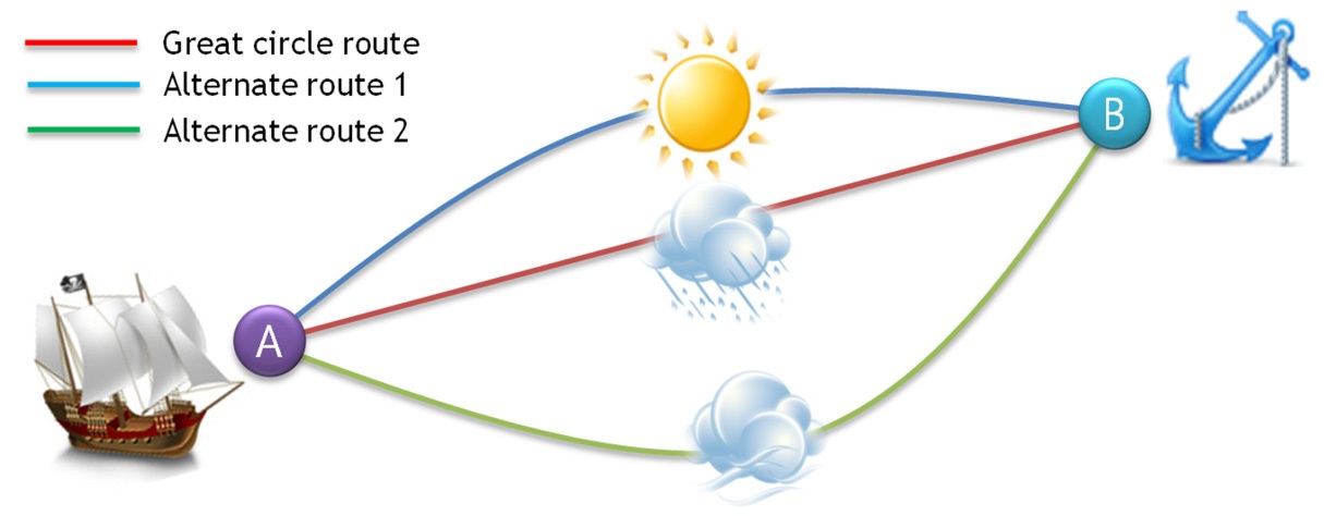
If the sea state of a great circle route (the shortest route connecting two points) is bad when a ship sails across the sea, there is a decision to make. It must be decided whether to continue sailing across the sea while running the risk of facing foul weather, or to change the original route and seek a safer but longer route with good weather.
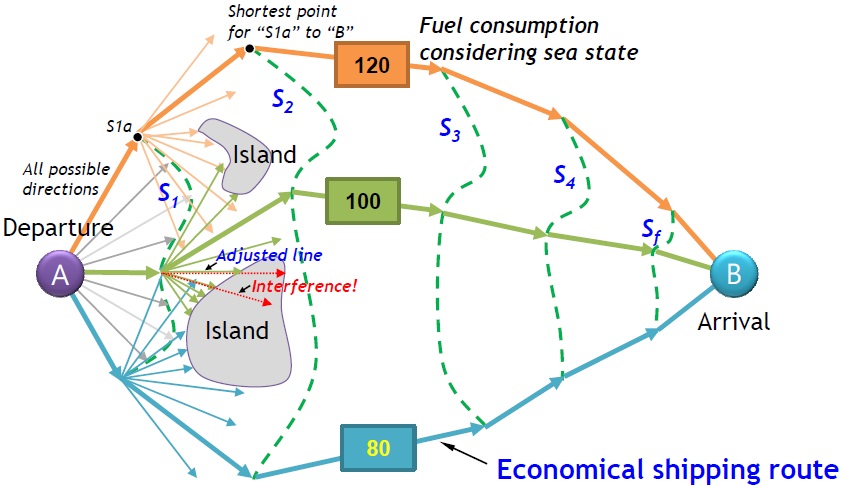
In the former case, additional fuel is consumed, because additional horse power is needed to compensate the speed loss of the ship in order to reach the destination on time, due to the increase in resistance of the ship due to the rough conditions. In the latter case, additional fuel is consumed because the distance to sail becomes longer than the original route, but there is no decline in the ship’s speed due to the sea state. Therefore, an economical shipping route can be determined if the fuel consumption for both cases is estimated and compared. The sailing time defined as the elapsed time from the start point to the end point can be used as an additional or alternate criterion for determining an economical shipping route. Fig. 1 shows an example.
The problem of determining an economical shipping route is an optimization problem. In this study, the problem is formulated mathematically as follows:


where:
X : ship route
TFOC (Total Fuel Oil Consumption) : total fuel consumption regarding applicable route
ETA (Estimated Time of Arrival) : estimated time of arrival regarding applicable route
ETAreq : required time of arrival (given value)
In this model, the design variable that must be found is the sea route of the ship. Formula (1) refers to the objective function, which suggests that the total fuel consumption regarding an applicable route should be minimized. Formula (2) refers to the constraint that a ship should arrive at the point intended within the required time.
METHOD OF ACQUIRING MARINE INFORMATION
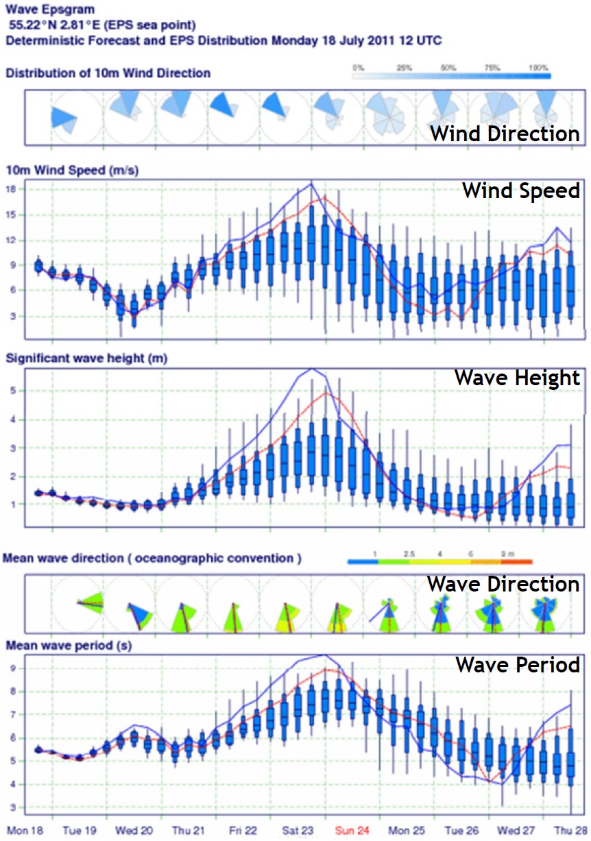
Satellite communication should be used to obtain real-time information for the sea state while at sea. Real-time marine information can be obtained from various sources. This study assumes that real-time marine information is obtained from the European Center for Medium-range Weather Forecasts (ECMWF) via satellite communication while at sea. The ECMWF was established with eighteen member countries in Europe with 142 experts who developed models, provided medium-range weather forecasts and weather data, and improved weather forecast techniques. The ECMWF provides long-term weather forecast data based on existing data as well as real-time marine information. 10-day weather forecast data is updated every 6
METHOD FOR ESTIMATING FUEL CONSUMPTION
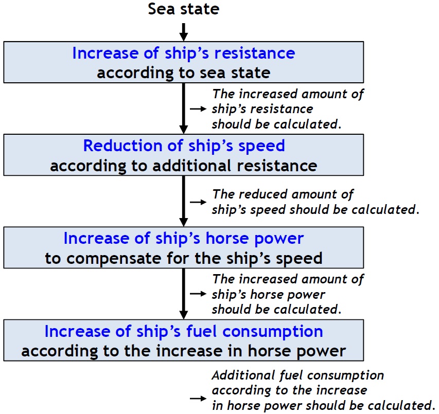
Fig. 3 shows the change in ship performance according to the sea state. With bad sea state (i.e. high waves), the total resistance of the ship increases. Ship speed also declines due to the rise in ship resistance, and additional horse power is needed to correct the reduced ship speed, which leads to additional fuel consumption.
In order to estimate fuel consumption according to the sea state, (1) first, the increased amount of ship resistance should be calculated. (2) Second, the reduced amount of ship speed according to the increase in ship resistance should be calculated. (3) Third, the increased amount of horse power to recover the ship speed should be calculated. (4) Lastly, the additional fuel consumption according to the increase in horse power should be calculated.
>
Calculation of additional resistance of a ship
To calculate the additional resistance of a ship, the ISO 15016 method (ISO, 2002) was used in this study. Using this method, the increased amount of ship resistance can be calculated according to the actual sea state, regarding the additional resistance relative to the resistance value of the ship in deep sea with no wind, waves, ocean current, and with a smooth hull and propeller surfaces. This information is used for interpreting the result of test runs by classifying the increased amount of ship resistance according to the actual sea state, characterized by the additional resistance comprising six items, as shown in formula (3):

where Δ
A ship usually encounters irregular waves during navigation. By making use of the response function of the ship in regular waves, the resistance increase of ships in short-crested irregular waves (Δ

where:
f : the frequency of the elementary incident wave (1/s)
G : the direction distribution of incidence waves
S( f ): the frequency distribution of incident waves (m2/s)
α : the direction of the elementary incident wave (rad)

: the response function of resistance increase in regular waves (N/m2)
The resistance increase due to wind (Δ

where:
CAA (φWR) = CAA0? K (φWR)
CAA (φWR) = the wind resistance coefficient
CAA0 = the wind resistance coefficient in head wind
K (φWR) : the directional coefficient of wind resistance
AXV : the area of maximum transverse section exposed to the wind (m2)
VWR : the relative wind velocity (m2)
φWR : the relative wind direction (rad)
ρA : the mass density of air (kg/m3)
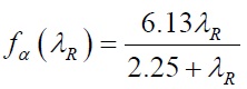
The resistance increase due to steering required by course keeping ( Δ

where:
AR : the rudder area (m2)
tR : the resistance deduction fraction due to steering
Veff : the effective inflow velocity to rudder (m/s)
δR : the rudder angle (rad)
λR : the aspect ratio of rudder
The resistance increase due to drifting (Δ

where:
ρ : the mass density of sea water (kg/m3)
d : the draft of ship (m)
V0 : the ship speed in stagnant water
β : the drift angle (rad)
The resistance correction value by the effect of water temperature and salinity ( Δ

where:
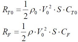
RT0 : the total resistance at contractually specified water temperature and salt content which may be derived from model tests (N)
CT0 : the total resistance coefficient for contractually specified water temperature and salt content
RF : the frictional resistance at actual water temperature and salt content in navigation (N)
CF : the frictional resistance coefficient for actual water temperature and salt content in navigation
CF0 : the frictional resistance coefficient for the contractually specified water and salt content
ρ : the water density for actual water temperature and salt content in navigation (kg/m3)
ρ0 : the water density for the contractually specified water and salt content (kg/m3)
S : the wetted surface area of ship (m2)
Finally, the resistance correction value by the effect of the difference in trim or draft of the ship (Δ

where:
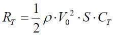
RT : the total resistance which may be derived from model test (N)
Δ : the displacement during navigation (ton)
Δ0 : the displacement as contractually specified (ton)
>
Calculation of the reduction of ship speed according to additional resistance
In this study, the reduced amount of ship speed according to additional resistance was calculated by calculating the interpretation of a test run that was provided by ISO 15016. This method calculates the changed amount of ship speed using formula (10):

where:
δV : the changed amount of ship speed by additional resistance
δVAR : the changed amount of ship speed by resistance increase
δVAC : the changed amount of ship speed by current
δVAA : the changed amount of ship speed by air resistance
δVAS : the changed amount of ship speed by shallow water
>
Calculation of the increase of horse power for correcting ship speed
Additional horse power is needed to correct a reduced ship speed to the initial ship speed. The increased amount of horse power that is needed to correct the ship speed is calculated using formula (11), which was proposed by Nakamura and Naito (1972), and formula (12) by Townsin and Kwon (1993):

where:
δ P: the increased amount of horse power needed to correct ship speed
N0P , Q0P : the number of propeller revolutions and amount of torque in stagnant water when the ship speed is V0
δQP , δNP : the increase in thrust and increase in the number of revolutions by the reduction in ship speed
where:
δP : the increased amount of horse power needed to correct ship speed
δV : the reduced amount of ship speed by additional resistance
V0 : the ship speed in stagnant water
n : a constant that varies according to the kind of ship
>
Estimation of additional fuel consumption according to the increase in horse power
The total fuel consumption for an applicable route can be estimated by formula (13):

where

where:
SFOC (Specific Fuel Oil Consumption) : fuel consumption ratio of main engines (g/hp·h)
δP: increased amount of horse power to correct ship speed
ETA (Estimated Time of Arrival) : estimated time of arrival regarding an applicable route
METHOD FOR DETERMINING ECONOMICAL SHIPPING ROUTE
>
Overview of the isochrone method
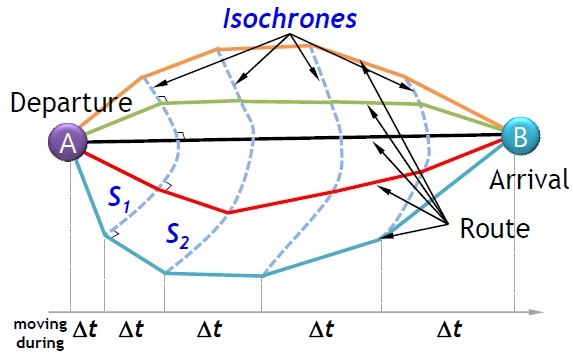
The isochrone method was proposed for manual use by a navigator for route planning. An isochrone is a set of connected points that a ship can reach within a given time limit starting from one point and going in all possible directions, as shown in Fig. 4. The points are dependent on the ship’s performance according to the sea state. The first isochrone (S1) shows possible routes for a given time limit from the point of departure. From each point belonging to S1, a perpendicular line to a tangent is determined in order to draw the second isochrone (S2). A segment of the line representing the distance that the ship can reach within the next time limit defines a point on S2. A set of such connected points forms S2. The next isochrones (S3, S4, …) are generated similarly.
>
Proposal of the improved isochrone method
While the isochrone method proposed by Hanssen and James can determine an economical shipping route in a short time with ease, there are difficulties in applying it to complex maritime areas. There are two main disadvantages of the method. The first is that this method is hard to apply to the determination of an economical shipping route with obstacles such as islands. The method does not consider interferences between isochrones and islands. The second is known as an “isochrone loop” (Wisniewski, 1991). Such a loop is an irregularity in the shape of an isochrone caused by the non-convexity of a ship’s performance for a given sea state. The isochrone loops propagate with the number of isochrones, and make the procedure inapplicable for determining an economical shipping route as a result. This study proposes a method that improves upon the existing isochrone method. To solve the first disadvantage, an interference check between the isochrones and islands is performed while determining a set of connected points for the next isochrone. To solve the second disadvantage, a segment of the line representing the distance that the ship can reach within the next time limit is not fixed to the perpendicular to the tangent of the isochrone. The overall algorithm of the proposed method is as follows. Fig. 5 shows an example of determining an economical shipping route whose fuel consumption is the lowest from the starting point to the point of arrival.
(1) Step 1: draw isochrones S1 by connecting points that can be reached within a given time limit, after considering obstacles through an interference check, and the sea state from the point of departure (A) to each direction determined by the user, as shown in Fig. 5. For example, in the case that there are obstacles such as land and an island in the applicable direction, going toward the direction is not possible. Then, the distance that can be reached within the time limit according to the sea state is determined by considering the reduction in ship speed and its correction.
(2) Step 2: find a point whose distance to the point of arrival (B) is the shortest among points that can be reached within the given time limit in each direction from each point on isochrones S1, and then make S2 by connecting them. As shown in Fig. 5, some lines for the given direction are interfered with by an island. These lines are adjusted and shrunk through intersection calculation.
(3) Step 3: draw isochrones by repeating step 2. Through the repeat of Steps 2 and 3, all isochrones of the first to the last isochrones can be made.
(4) Step 4: connect points on Sf , the last isochrones, and the point of arrival.
(5) Step 5: calculate fuel consumption according to routes and then determine the route whose fuel consumption is the lowest as an economical shipping route.
>
Comparison of performance with existing algorithm
In this study, the performance of the improved isochrone method is compared with the A* algorithm (Jung and Rhyu, 1999) in order to verify the efficiency of the improved isochrone method.
A* algorithm
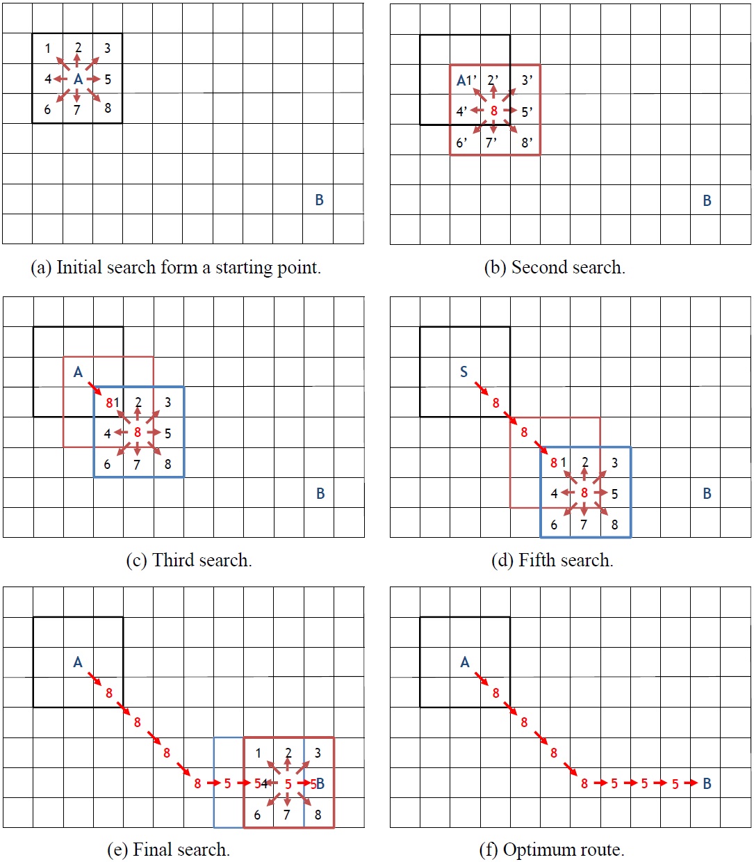
The A* algorithm is a graph search algorithm that searches for a route from an initial node (starting point) to an objective node (point of arrival). As shown in Fig. 6(a), there are 8 directions that can be searched from one point. 8 nodes (node 1 - node 8) can be reached from point A, which is the starting point. Node 8 is stored in a search list, since it is the closest to B, which is the point of arrival. 7 nodes (node 1 - node 7) are stored in a candidate list according to their proximity to the point of arrival. Once a search is done at node 8, node 8’ is stored in the search list, and then the remaining nodes (node 1’ - node 7’) are stored in the candidate list according to their proximity to the point of arrival (see Fig. 6(b)). The shortest route from the starting point to the point of arrival can be found by applying this process to nodes that were stored in search list (see Fig. 6(f)). The A* algorithm can be applied to complex maritime areas that have many islands, but it requires considerable memory and time since it inspects all areas one by one.
Comparison of performance through examples
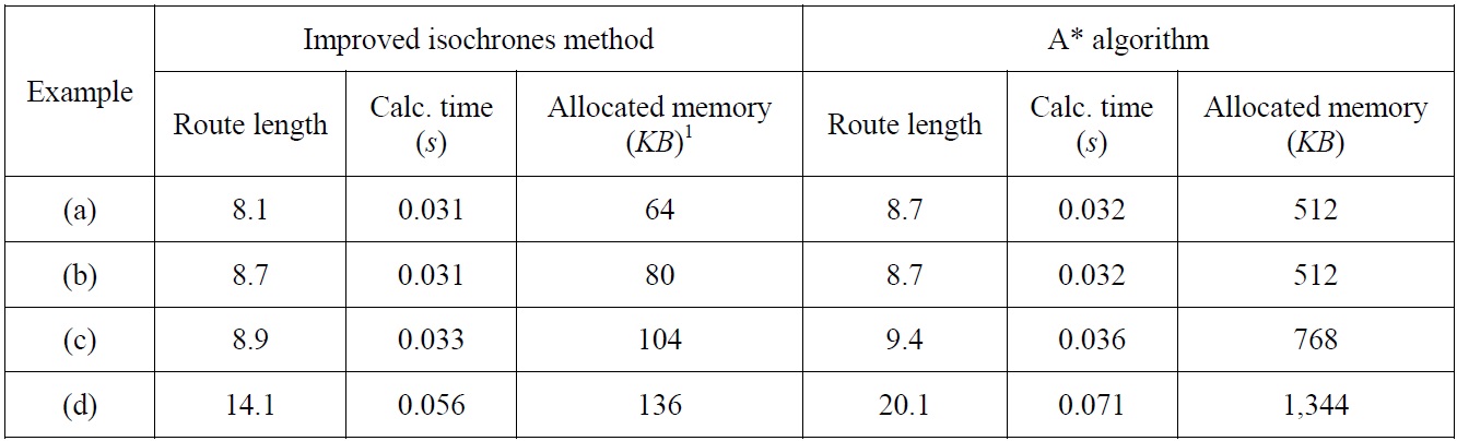
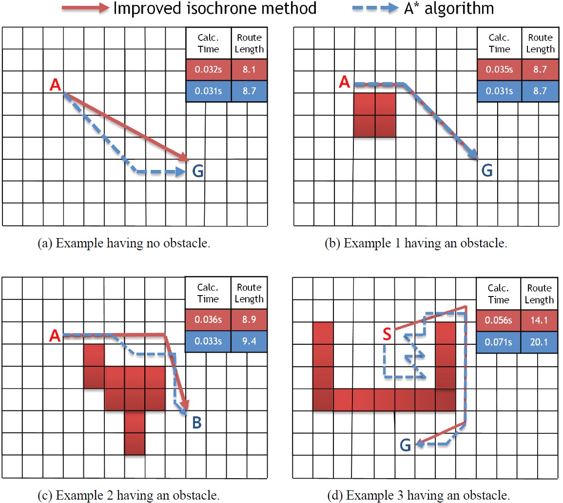
The results of the performance comparison with the A* algorithm for simple examples are summarized in Fig. 7. As shown in Fig. 7(a), the A* algorithm finds a route whose distance is somewhat longer than that of the isochrone method, because the A* algorithm searches focus on neighboring nodes. Table 1 shows the calculation results for the examples using the two methods.
[Table 1] Comparison of the improved isochrone method with the A* algorithm for 4 examples.

Comparison of the improved isochrone method with the A* algorithm for 4 examples.
EXAMPLES OF DETERMINING ECONOMICAL SHIPPING ROUTE
A Very Large Crude oil Carrier (VLCC) with 270,000
>
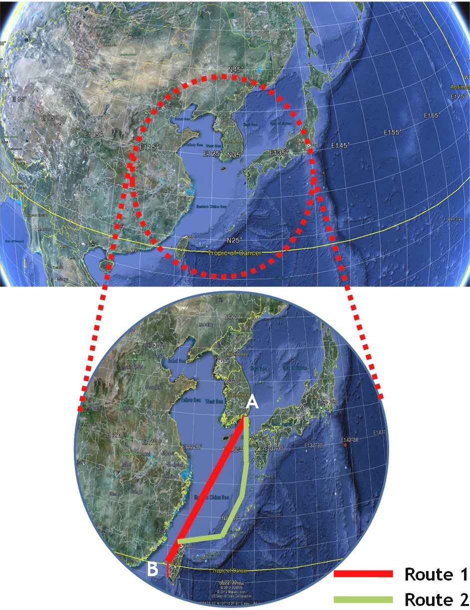
Application to short-distance route from Korea to Taiwan
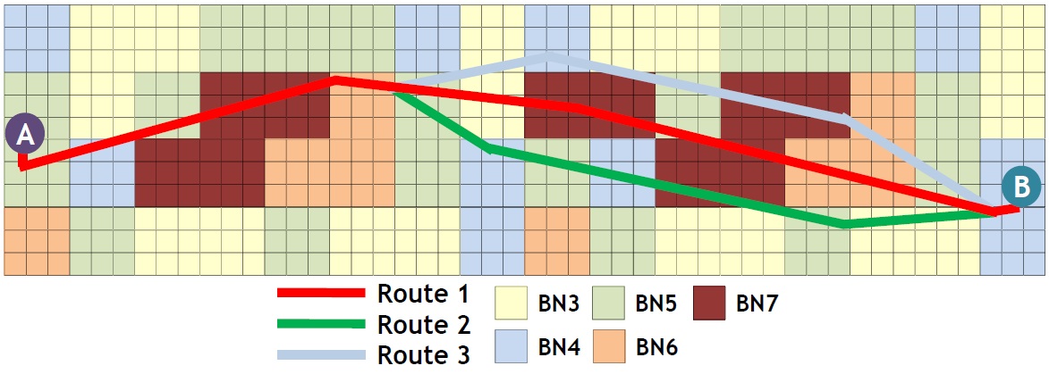
As shown in Fig. 8, the first applied route covered areas among ship routes from Busan in Korea to Kaoshsiung in Taiwan, which is a relatively short route. Data provided by ECMWF were used for the sea state of the areas. Marine information was expressed as Beaufort Number (BN) for convenience. BN is an index that indicates the sea state, with a greater value corresponding to a worse sea state.
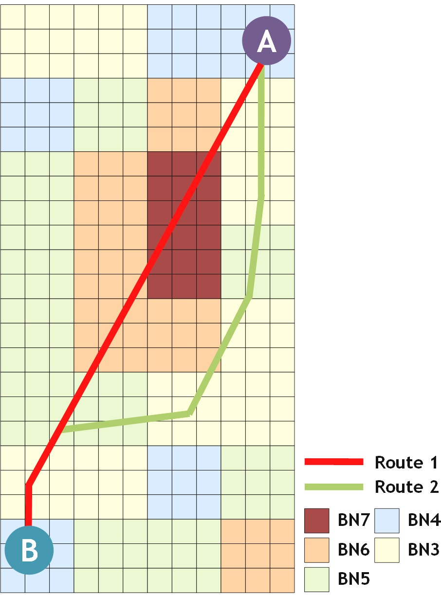
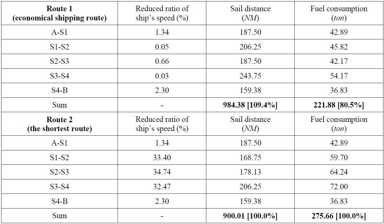
In this example, it was assumed that a ship passes between A and B, where the sea state is bad (marked as an ellipse in Fig. 8). Various routes were searched based on the improved isochrone method (see Fig. 9), and an economical shipping route was determined by estimating the fuel consumption for two routes among various routes. The route from A to B was divided into isochrone sections with a certain time, and then fuel consumption was estimated by calculating the additional resistance of the ship, the reduction of ship speed, and the additional horse power, by considering the sea state for each section. Table 2 shows the result of estimating fuel consumption for each sea route.
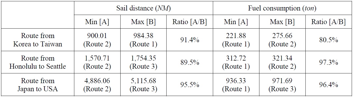
As shown in Table 2, ship route 2 provides the shortest distance amounting to 900.01

Result of determining an economical shipping route using the improved isochrone method for the route from Korea to Taiwan.
>
Application to medium distance route from Honolulu to Seattle
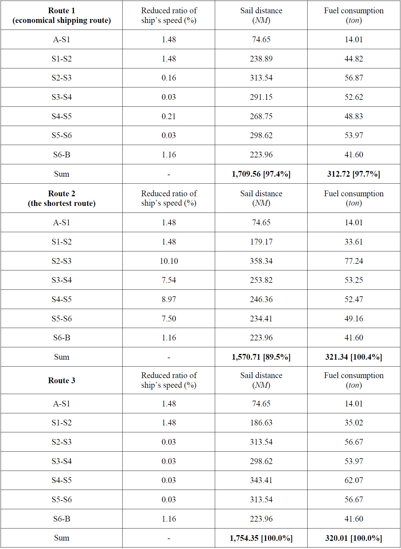
Next, the proposed method is applied to a medium-distance route from Honolulu to Seattle in the USA, as shown in Fig. 10. Data provided by ECMWF was also used for the sea state of the areas. Similarly, it was assumed that a ship passes from A to B, where the sea state is bad in this example. Various routes were searched based on the improved isochrone method (see Fig. 11), and an economical shipping route was determined by estimating the fuel consumption for three routes among various alternatives. As shown in Fig. 11, the route from A to B was divided into isochrone sections with a certain time, and then the fuel consumption was estimated by considering the sea state for each section. Table 3 shows the result of estimating fuel consumption for each sea route.

Result of determining an economical shipping route using the improved isochrone method for the route from Honolulu to Seattle.
As shown in Table 3, ship route 2 provides the shortest distance of 1,570.71
>
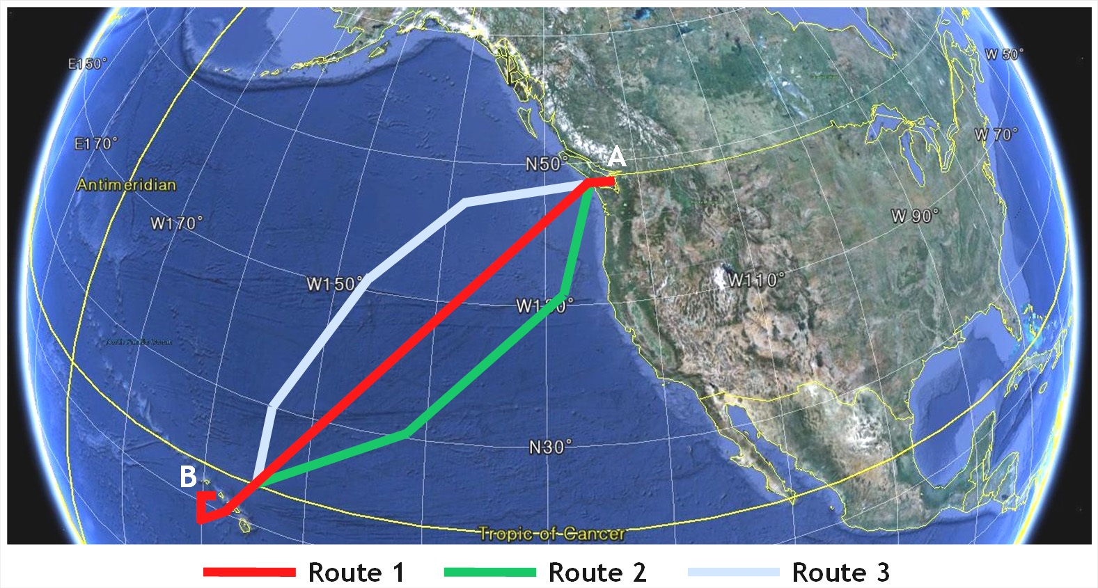
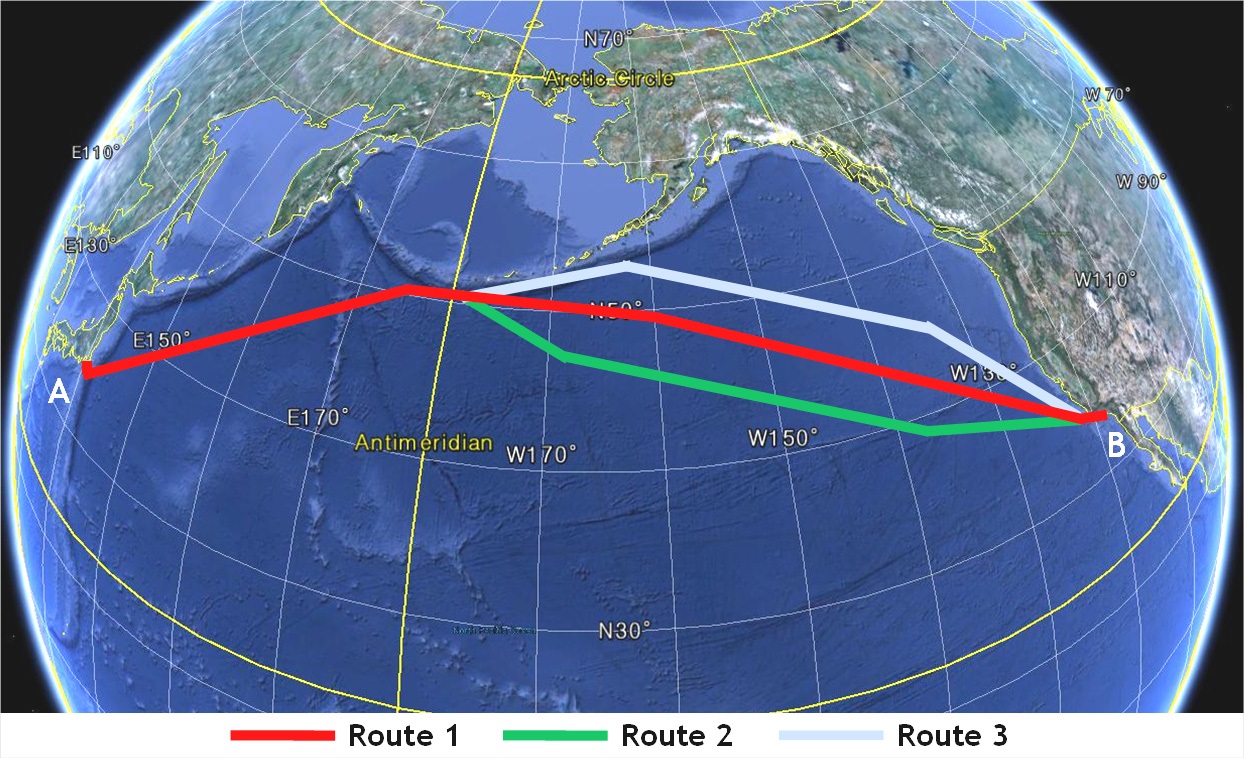
Application to long-distance route from Japan to USA
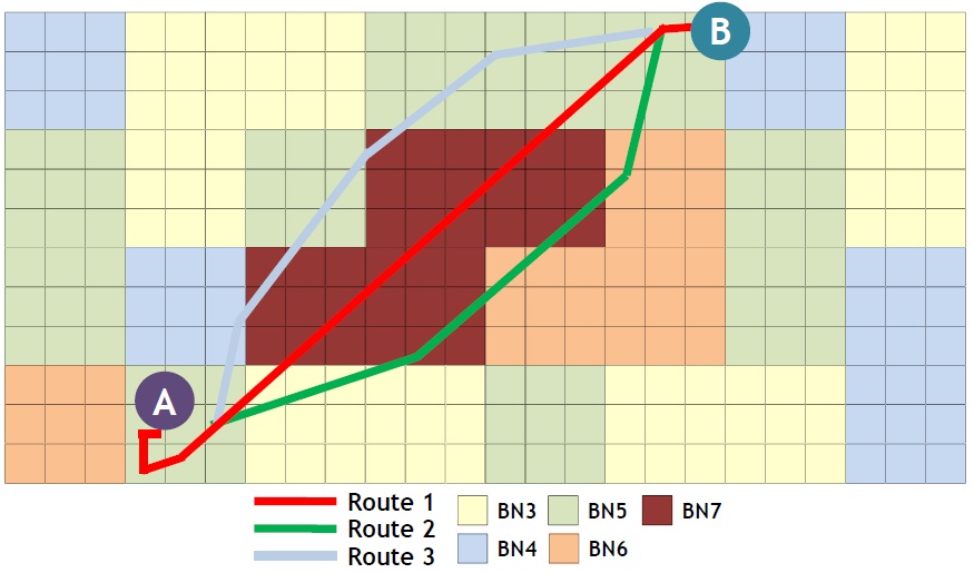
The final example is for a long-distance route from Yokohama in Japan to Long Beach in the USA, as shown in Fig. 12. Similarly, it was assumed that a ship passes between A and B, where the sea state is bad in this example. Various routes were searched based on the improved isochrone method (see Fig. 13), and an economical shipping route was determined by estimating the fuel consumption for three routes among various routes. As shown in Fig. 13, the route from A to B was divided into isochrone sections with a certain time, and then the fuel consumption was estimated by considering the sea state for each section. Table 4 shows the result of estimating fuel consumption for each sea route.
As shown in Table 4, ship route 2 provides the shortest distance of 4,886.06
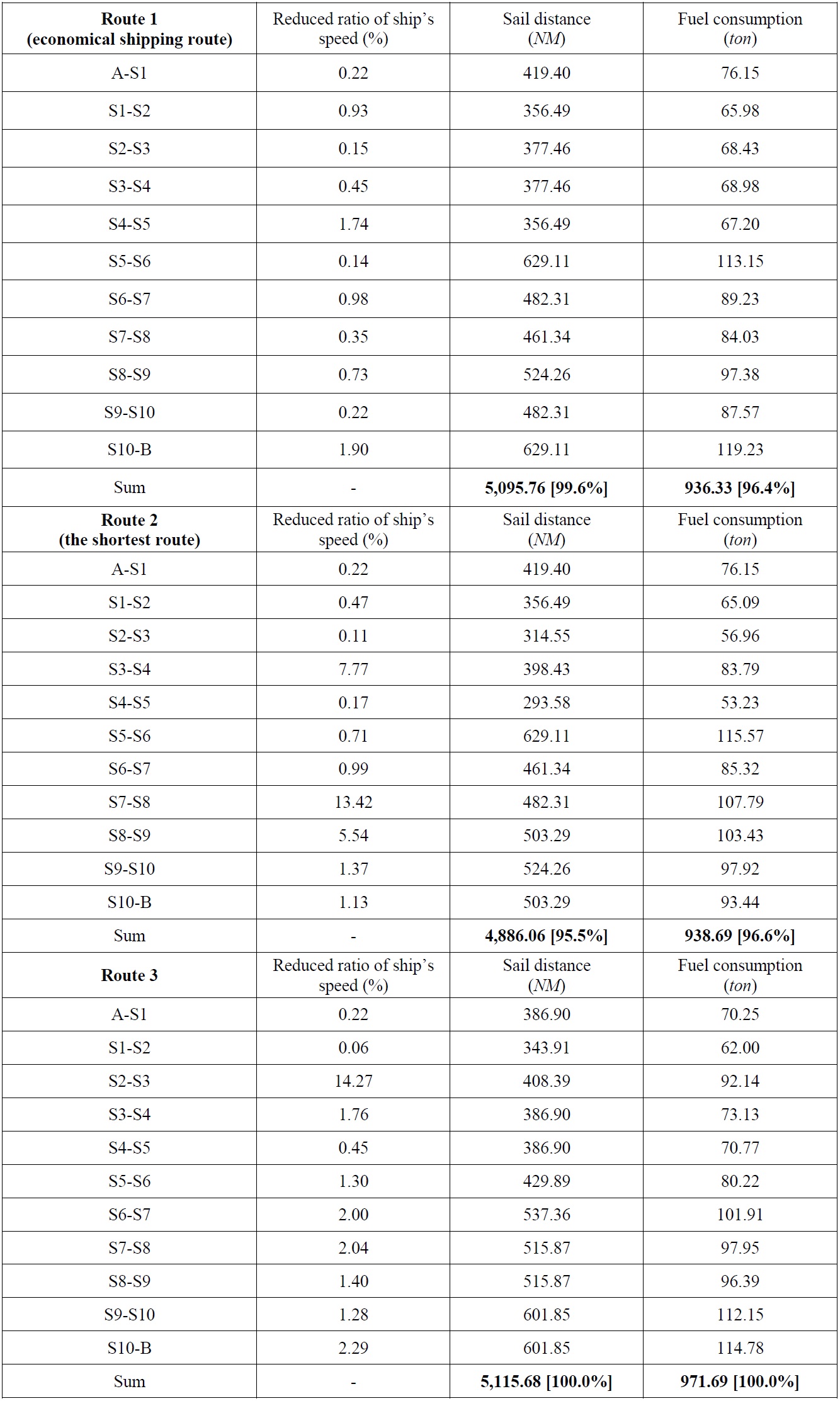
Result of determining an economical shipping route using the improved isochrone method for the route from Japan to USA.

Comparison of the results of determining an economical shipping route using the improved isochrone method.
This study was conducted to find a way to determine economical shipping routes based on real-time marine information and the estimation of fuel consumption. Marine information was obtained from ECMWF, and the additional resistance applied to ships according to the sea state was estimated, based on which the additional horse power to correct the reduction in ship speed was estimated. Then, the fuel consumption of the ship was estimated. Based on these calculations, an economical shipping route was determined using the improved isochrone method. The findings were applied to actual maritime areas in order to verify the efficiency of the method. Plans have been made to improve the reliability and utility of the proposed method by studying ways to estimate fuel consumption more precisely, and applying the findings to more practical examples in the future. Particularly, to improve the estimation of fuel consumption, a method of using actual operating data from shipping companies will be investigated and incorporated into the proposed method.