As the demand of natural resources such as natural gas and oil are tremendously increased, the huge size carrier such as liquefied natural gas (LNG) carrier is fabricated in nowadays. In accordance with this phenomenon, a lot of risk factors such as sloshing problem, crack propagation problem in midship section are emerged. Among these, the sloshing problem is considered as one of the most catastrophic problems since the structural failure of the LNG carrier leads to not only leakage of LNG but also tremendous loss of human and financial resources.
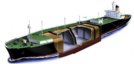
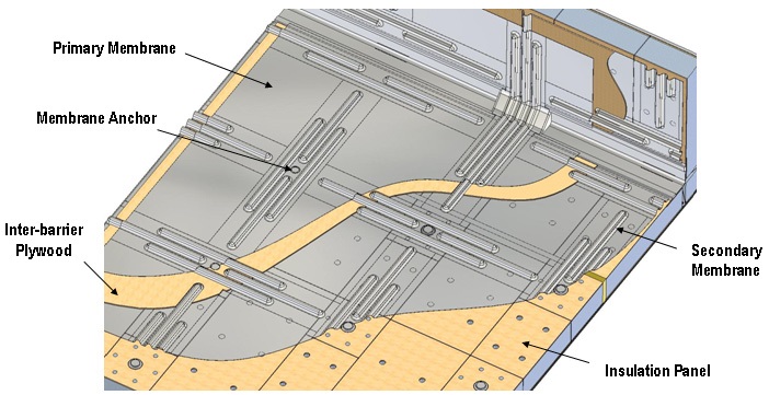
In order to overcome this problem, i.e., the insulation system which is consisted of lots of composites and austenitic stainless steels is adopted such as MARK-III-type, NO-96-type, KC-1-type insulation system. Among these, the KC-1-type insulation system which is fabricated by shipbuilding companies of Korea is designed to sustain the leakage of LNG as well as structural failure. Figs. 1 and 2 show the schematic of the membrane-type LNG carrier and the KC-1-type insulation system. This insulation system encounters the severe sloshing loads during its oversea operation. Hence, it is essential to guarantee the structural safety of the insulation system during its design and fabrication.
For several decades, the hydroelastic analysis under sloshing has been analyzed by computational methods. In other words, the hydrodynamic pressure distributions as well as wave characteristics near the boundary condition are successfully evaluated based on finite element method (FEM) (Valtinsen, 1974; Nakayama and Washizu, 1980; Wu et al., 1998). However, in these researches, the structural response and behavior is not focused on, because the container is postulated as a rigid body and the interactive effect between interior fluid and exterior container is ignored. It is considered that the tremendous computational time and cost would be demanded when the structural deformations and interactive methods are adopted.
As an alternative method, the global-local basis fluid-structure interaction (FSI) analysis has gained attention for addressing the sloshing-induced structural response problem (Mote, 1971; Mao and Sun, 1991; Cho and Lee, 2003; Cho et al., 2008). In these researches, the structural behavior as well as correlation between internal LNG flow and external container can be considered in a unified formulation. On the other words, the sloshing-induced flow and hydrodynamic pressure can be obtained during the global analysis. In addition, the structural stress/strain and deformation can be estimated during the local analysis. In the process of the local analysis, the container is considered as a deformable body (not a rigid body) and boundary/initial conditions at an arbitrary time are implemented into the local analysis procedures. For this reason, the computational time and cost can be saved during the global-local analysis process.
Hence, in the present study, the global-local method based hydroelastic analysis which is successfully derived by Cho et al. (2008) has been adopted to evaluate the structural safety as well as hydrodynamic pressure induced by interior LNG flow for the KC-1-type LNG insulation system. During the global analysis, the flow motion characteristics such as the flow velocity, hydrodynamic pressure and volume fraction which are used as an initial and boundary condition for the local analysis are obtained. In addition, during the local analysis, the structural behaviors of the actual sized KC-1-type insulation system such as effective stress/strain and deformation are estimated precisely.
NUMERICAL MODELING OF HYDROELASTIC PROBLEM FOR LNG CARRIER’S INSULATION SYSTEM UNDER SLOSHING
>
Description of numerical modeling
The aforementioned hydroelastic problem has been analyzed by many scientists and engineers (Morand and Ohayon, 1995), especially Cho et al. (2008) who have successfully solved the hydroelastic problem of the MARK-III type LNG insulation system under sloshing. Prior to the FSI analysis for the KC-1-type LNG insulation system, the theoretical backgrounds such as problem descriptions, global-local analysis method are discussed in Chapter 2 based on the authors’ previous study (Cho et al., 2008).
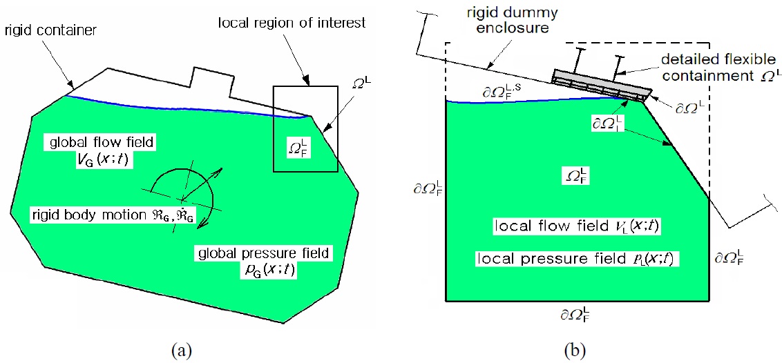
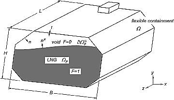
The hydroelastic response problem of the LNG carrier’s insulation system is a representative example of the FSI problem, namely, the deformation of the insulation system (structure) is induced by LNG sloshing (fluid). Fig. 3 shows the LNG carrier’s insulation system with length
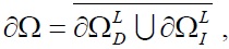
By considering the insulation system as a three-dimensional linear elasticity, the material and boundary domain can be written as Ω∈R3 and
respectively, where ∂Ω


where

are the initial value of the displacement and velocity fields, respectively. u denotes the displacement constraint by the rigid dummy closure, which moves by the rigid body motion of the global rigid container.
The LNG domain transformed into the movement of the free surface ∂Ω

The momentum equation can be written as follows.

The initial and boundary conditions of Eqs. (5) and (6) can be represented as


where

acting on the LNG-free boundary disappears when the flow is assumed to be inviscid (Cho and Lee, 2003). The total stress tensor of LNG
The flow boundary can be used to obtain the transport equation and its initial condition; namely,


where
>
Global-local analysis technique
In order to analyze the structural response of complex structures, a huge number of degrees of freedom are needed; hence, a large amount of computational time and cost is required. Thus, it is impossible to obtain the structural response for the entire structure as a whole. The global-local analysis technique was introduced as an alternative method to investigate the structural response of regions of interest in structures (Mote, 1971; Mao and Sun, 1991). In global-local analysis, the global analysis is carried out prior to the local analysis. The finite element (FE) model is simplified to save the calculation time. By using approximate mechanical information of the global structures such as the reaction force, the displacement can be obtained. Based on this information, local analysis of the region of interest is then performed. In local analysis, the FE model is fabricated as a real structural/material model, and specific mechanical information of specific regions can finally be acquired. The global-local analysis technique is widely used in the structural analysis of complex structures due to its reliable analysis results and efficient computational time/cost.
Fig. 4 shows the global-local approach for the hydroelastic analysis. The structural response of the right-top corner region of the LNG insulation system was investigated at critical time
In local hydroelastic analysis, the continuity and momentum equations can be written as


where V


The transport equation and its boundary condition can be written as


where

can be ignored due to the assumption of inviscid flow.
The undamped displacement u
where ∂Ω

The initial and boundary conditions of the above equation can be expressed as


where R
>
Numerical approximation for FVM-FEM coupling
Eqs. (12), (13), and (16) can be represented by a generalized form, that is,

where Φ is the dependent variable, Λ is the coefficient,

is the extended Euler region including the void region within the local insulation system. In other words, Φ=1, Λ =
is discretized into a finite number of non-overlapping control volume, and the time period
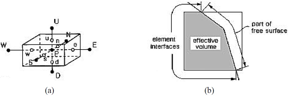
Fig. 5(a) shows the three-dimensional control volume of grid point

at time stage

Here,

is the volume integral of the source term

where

is the part of
independent of Φ,

is the coefficient of Φ
and
are the coefficients at arbitrary time step
From Eq. (24), the discretized formula to obtain the variable

at time step

where
The momentum equations in the discretized linear algebraic equations system, i.e., Eq. (25) are firstly solved to compute time-step-wise flow velocities using the initial conditions or the previous time-level values. It is evident from Fig. 5(b) that volume and surface integrals of the partially filled elements are carried out over the effective volume and the effective boundary, respectively, where the effective boundary consists of the element interfaces and the part of the fluid free surface.
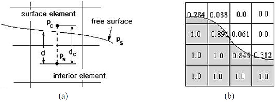
On the other hand, the calculated velocities do not satisfy the continuity equation, hence, the pressures should be adjusted in each control volume element occupied by the fluid. From Fig. 6(a), the element-centered pressure

with
Once the pressure and velocity fields are calculated, the volume fraction equation in the discretized linear algebraic equation system, i.e., Eq. (25) is calculated to compute the element-wise constant volume fraction as shown in Fig. 6(b). In addition, in order to maintain the computational stability, the time-step size should not exceed the critical value given by

where
By applying the isotropic finite element approximation technique to Eq. (18), the undamped displacement field u

where ?

where F is the load vector by gravity and hydrodynamic pressure; this is written as follows.

The time integration is carried out based on the central difference method (explicit method) and/or Newmark method (implicit method). However, the explicit method is widely adopted in dynamic structural problems of huge/complex structures due to the reduction of analysis time (Hu, 1997). The local analysis time


According to the central difference method and dynamic relaxation method, which is based on the α-damping method, the velocity and displacement of each time step are derived as


where

where
On the other hand, in the local hydroelastic problem, the LNG flow and structural motion influence each other at the common surface ∂Ω


The fluid-structure constraints can be numerically represented by direct standardization and the iterative discretized method. Applying the former method to complex structures is extremely difficult. Therefore, the latter method was adopted for this study. The two kinds of equations (i.e., fluid domain and structure domain governing equations) are separately calculated by using the iterative discretized method, and the interaction of the fluid and structure is calculated alternately. In order to overcome the mismatch of the mesh, the projection method was also adopted (Farhat et al., 1998).
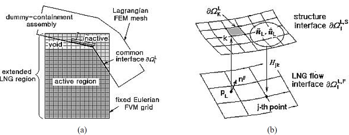
In the local analysis for this study, the fixed Eulerian mesh was used for the LNG flow, and the complex and dense mesh was used for structures. In this case, the incompatible Eulerian-Lagrangian interaction method can be used effectively. As shown in Fig. 7(a), the fluid mesh is larger than the physical domain of LNG, and the active and inactive domains are separated by the common interface ∂Ω
In order to transfer the hydrodynamic pressure

of the structure to the flow field, the related variables must be interpolated. In this study, the structure mesh was denser than the fluid mesh; hence, the mesh pattern and basic function of the structure can be used as a standard mesh to interpolate the related variables. As shown in Fig. 7(b), the surface force

which is transferred to the surface element ∂Ω

, is implicitly interpolated as


where
which is transferred from

and

is the two-dimensional master element.
The displacement and velocity of structure are transferred to the flow field using the incompatibility interpolation method (Harder and Desmarais, 1972). Here, note that the former adjusts the flow boundary of LNG, whereas the latter one specifies the flow boundary condition given in Eq. (15). In Fig. 7(b),
and
. Eq. (35), that is, the kinematic constraint, can be written as follows using the

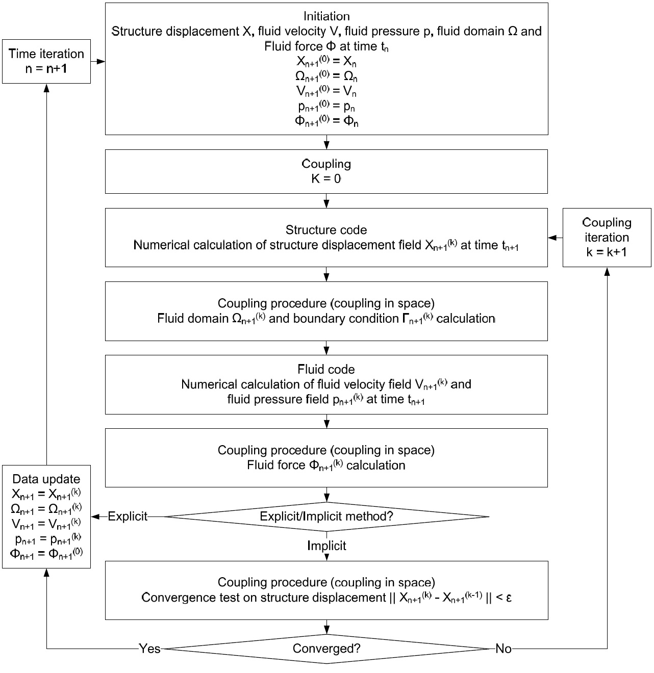
The coupling in time can be done using either explicit or implicit approach, and the flowchart of the analysis algorithm in both approaches is presented in Fig. 8 (Cho et al., 2008). Based on the analysis algorithm, the user-defined subroutine is programmed. In this study, the explicit time coupling for the current problem with the critical time-step size determined by Eq. (27)
and (34). The numerical implementation of the local staggered hydroelastic analysis using the explicit incompatible Eulerian- Lagrangian coupling method is carried out as follows.
(1) The initial structure-LNG interface ∂ΩLI in the local model is specified and the initial free surface
is defined by assigning the volume fraction FL to each local Eulerian cell.
(2) Based on initial and boundary conditions, i.e., Eqs (19)-(21), the structural dynamic equation system, namely, Eq. (18) is time integrated to solve the displacement uL and the velocity

of the local flexible insulation system.
(3) Next, the LNG interface
is moved by uL and specified with
as the interface flow boundary condition, i.e., Eq. (15) according to non-matching interpolation scheme, namely, Eq. (38).
(4) Based on the adjusted active LNG material boundary, the flow boundary conditions and the initial condition, i.e., Eq. (14), the transport equations (Eq. (22)) are solved to find the local flow velocity VL, the volume fraction FL, and the hydrodynamic pressure pL.
(5) The free surface
and the structure-LNG interface ∂ΩLI are updated, and then the LNG hydrodynamic pL is transferred to the structure interface
. And then, go to the next time integration.
DESCRIPTIONS OF KC-1 TYPE INSULATION SYSTEM FE MODELS
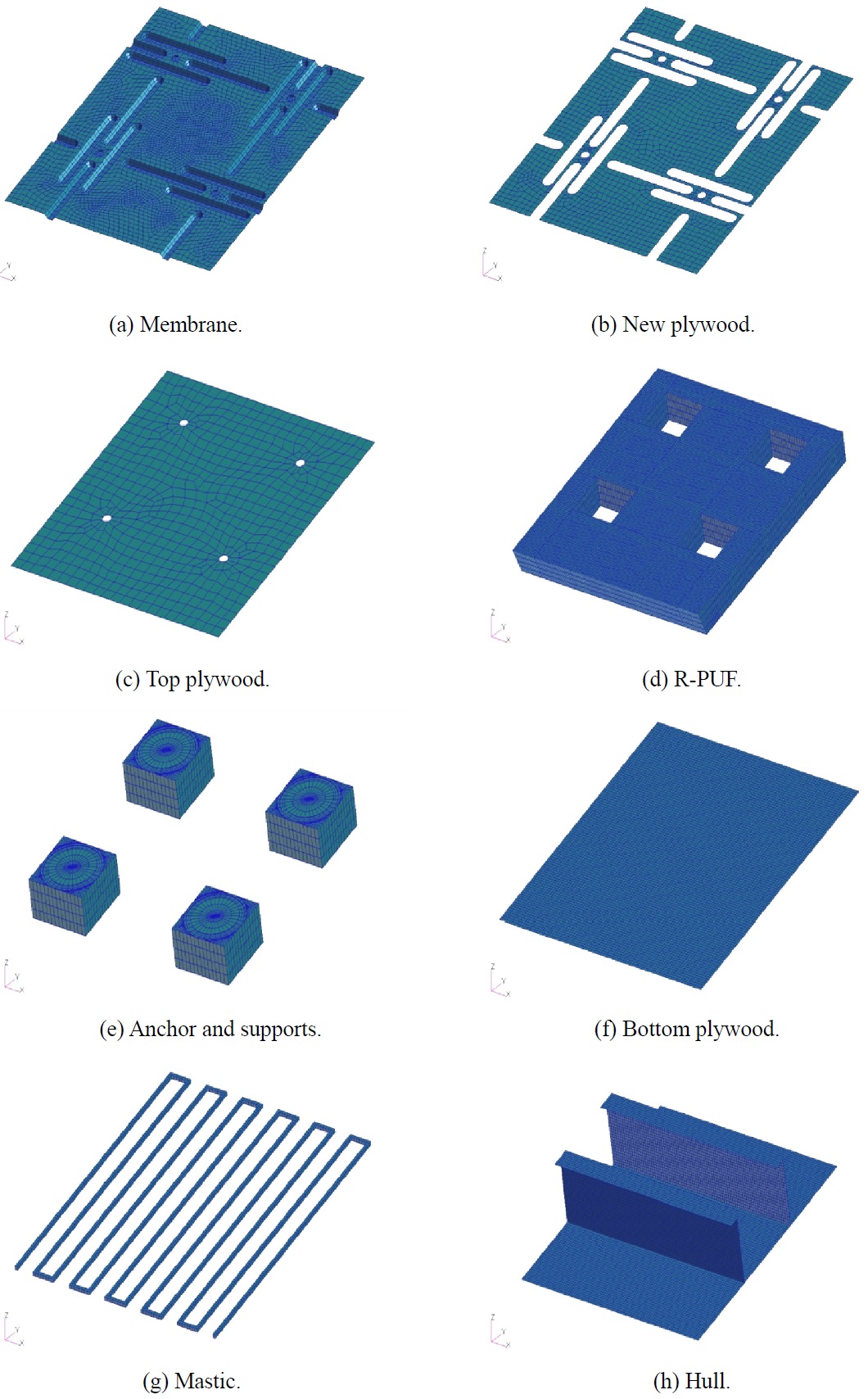
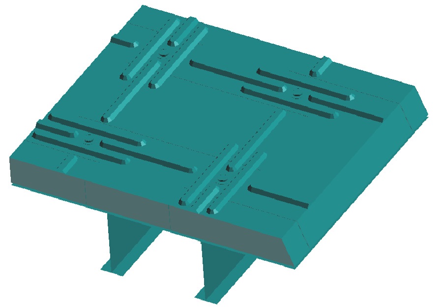
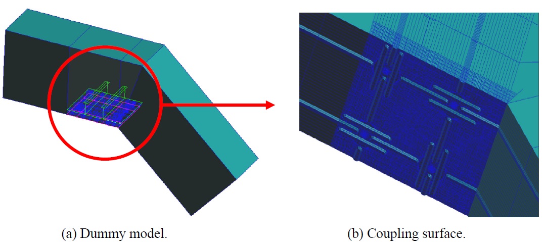
Figs. 9 and 10 show the local FE model and its component for the KC-1 type LNG carrier’s insulation system. Fig. 11(a) shows the dummy element used as an interface, and Fig. 11(b) shows the coupled interface between the dummy and the membrane of the insulation system. The mechanical properties and element type of the KC-1 type FE model are shown in Table 1.
[Table 1] Material properties and element type of KC-1 type model.
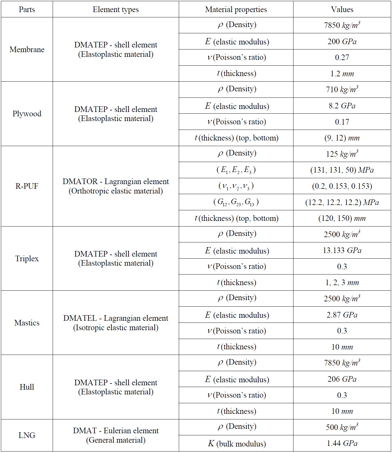
Material properties and element type of KC-1 type model.
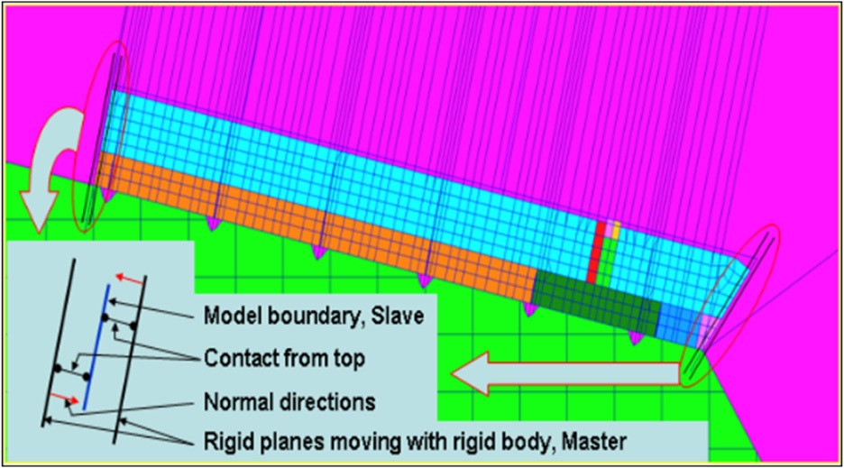
Fig. 12 shows the boundary conditions of the dummy-local KC-1 insulation system model. If node sharing is applied to this model, the stress concentration may occur on the interface between the dummy and local model. In other words, the model types of the dummy and local models are rigid and deformable, respectively. Hence, the mismatch in deformation can cause an abnormal increase of stress. In order to overcome this problem, the contact element was adopted between the two models used in this study.
>
Simplified FE model for anchor section
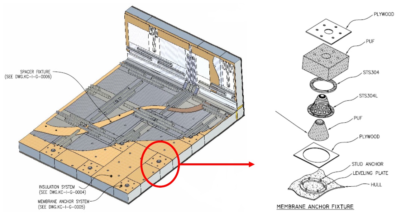
An anchor section exists between the insulation system and hull. The anchor combines the R-PUF and membrane firmly. The surface of the anchor is made of SUS 304L, and inside is filled with R-PUF. The implemented position and lamination structure of the anchor is shown in Fig. 13.
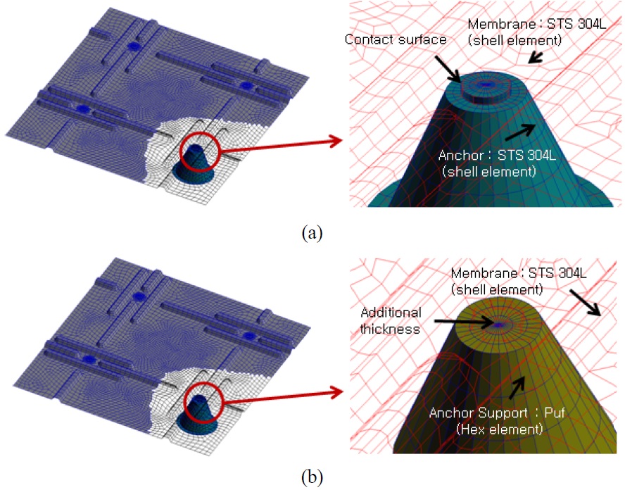
The anchor has extremely complex lamination structures, as well as others, and it might be necessary to create a mesh that is quite fine. However, this could induce a huge amount of calculation time to analyze the anchor region. In order to save the computational time and cost, the simplified FE model of the anchor section was introduced in this study. The two kinds of analysis scenarios were adopted as shown in Fig. 14.
Case A is the general FE model, which was fabricated by using element refinement. The connection area between the membrane and anchor was established as surface-to-surface contact. On the other hand, in Case B, the upper side of the anchor was eliminated for fast calculation. Instead, the additional thickness model with a coarser mesh size than the as-is model was implemented to the upper side of the anchor. In addition, this model was unified with the membrane FE model. By using the additional thickness model, the calculation time can be improved. Moreover, the modeling time can be reduced due to the absence of the contact element. The related description such as number of elements and computational time will be discussed in Chapter 4.
GLOBAL-LOCAL HYDROELASTIC ANALYSIS RESULTS AND DISCUSSIONS
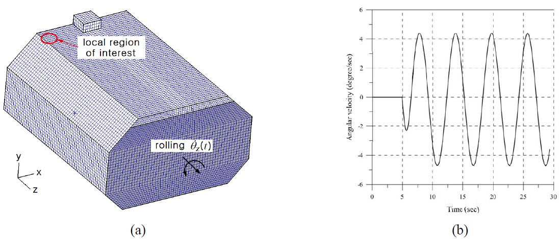
Fig. 15 shows the FE model of the LNG carrier insulation system for global analysis. The dimensions of the FE model were 42.84
The insulation system was applied to a sinusoidal rolling excitation as shown in Fig. 15(b). The angular velocity was defined as
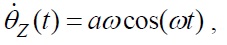
and the amplitude and the angular frequency were defined as a=3.87° and ω=2π/5.5
The computational analysis time was set to 0

= 3.598×10⁻³
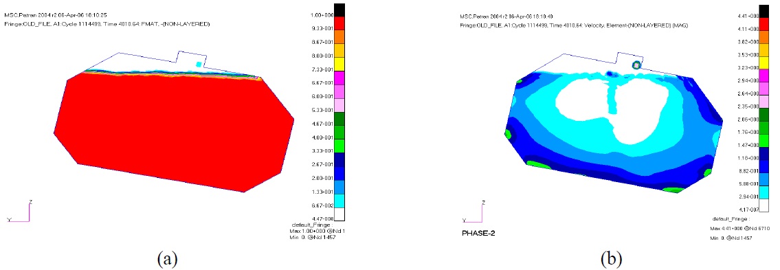
Fig. 16(a) and (b) show the volume fraction distribution and the sloshing flow of interior LNG at time 4010
It is noted that the insulation system experiences the peak rolling amplitude equal to 22.1° in the rigid tank sloshing. Although the excitation from 5 to 30
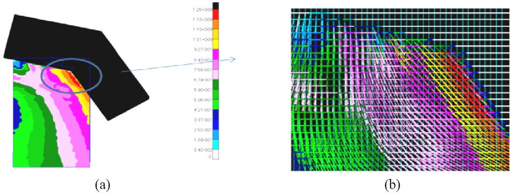
Fig. 17 shows the mapping of the LNG flow into the local problem region Ω
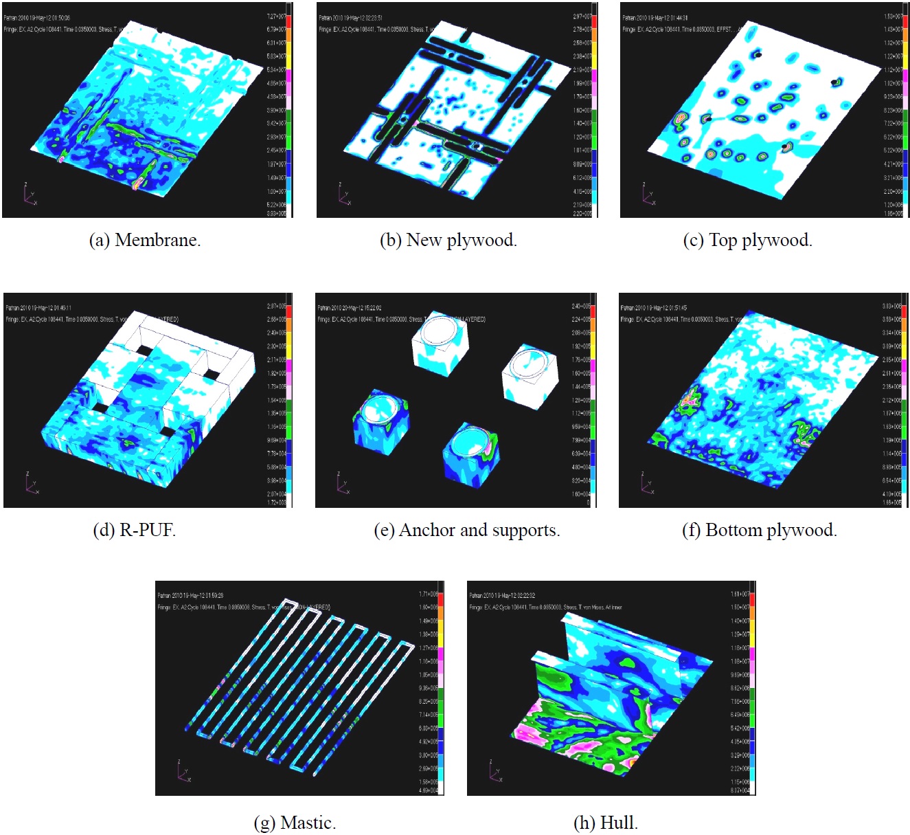
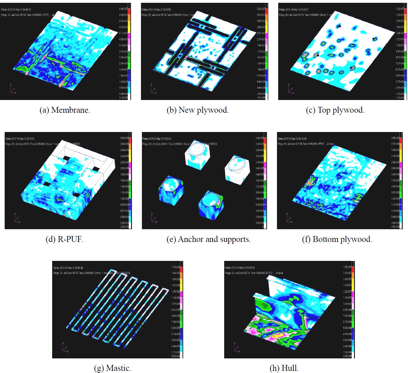
Based on the data of the global analysis results, the local analysis was carried out. Figs. 18 and 19 show the local analysis results of the effective stress contour regarding Cases A and B. In both cases, the maximum effective stress occurred in the membrane region at 35
Through Table 2, it is confirmed that the average stress value of Case B is bigger (but not much) than the value of Case A. It is considered that this phenomenon might be caused by the differences of element types, i.e., shell-contact element type in Case A and shell-hexahedral element type in Case B. However, these differences can be acceptable considering the computational time and cost as shown in Table 3. In this table, it can be found that the CPU time of Case A is much bigger than the Case B. Since it takes huge time to calculate the interface and contact regions in the Case A FE model. Hence, it is confirmed that the proposed FE model is more time and cost effective case when the FSI analysis of the LNG carrier cargo tank is carried out.
[Table 2] Maximum effective stress at 35 ms (local time) and 4010.035 sec (global time) (Unit: MPa).
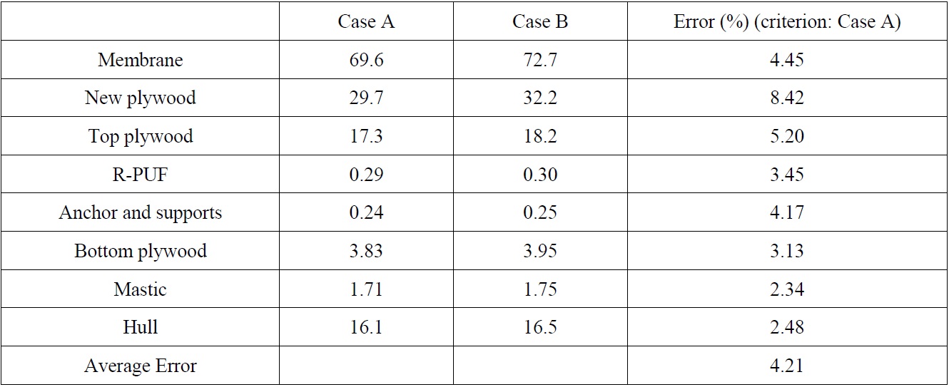
Maximum effective stress at 35 ms (local time) and 4010.035 sec (global time) (Unit: MPa).
[Table 3] Computational time for Case A and Case B.
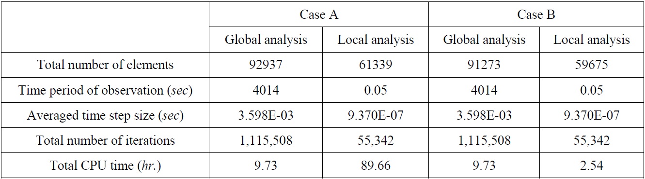
Computational time for Case A and Case B.
In this study, the sloshing resistance performance for the KC-1 type LNG carrier insulation system was evaluated by FSI analysis. The research results are listed below.
(1) FSI analysis was carried out based on the well-known arbitrary Lagrangian-Eulerian method, and other novel techniques for FSI analysis were introduced.
(2) The flow velocity, pressure, and volume fraction of the internal LNG of the KC-1 insulation system can be calculated during the sufficient sloshing time based on the global analysis method. The obtained values are mapped into the local FE model of the KC-1 insulation system.
(3) The maximum effective stress contours can be calculated based on the local analysis method. During local analysis, the arbitrary Lagrangian-Eulerian method based FSI analysis is adopted. Moreover, a novel element model, i.e, additional thickness model without contact element, was implemented into the local KC-1 insulation system in order to remarkably reduce the computational time and cost.
(4) Although validation of the analysis results through a comparison of the experiments was not carried out, the proposed analysis technique can potentially be used as a robust integrity assessment technique for LNG carrier’s insulation systems.