The management of spent fuel (SF) or transuranic (TRU) elements is the main goal for the generation of sustainable nuclear power. In this context, Generation-IV (Gen-IV) reactor systems are being developed. The Gen- IV systems aim at extensively increasing the safety and economics, and drastically minimizing the radioactive wastes [1]. Among the proposed Gen-IV reactor concepts, a sodium-cooled fast reactor (SFR) is being widely studied due to its capacity of fully recycling fissile plutonium and other TRU elements. The full-fissile plutonium and, in principle, TRU recycling is achievable in a fast reactor system through internal fissile breeding and the external reprocessing of SF, which enables an extension of the use of natural uranium resources and a reduction in waste production.
In this study, some mixing strategies of the low and high conversion ratio (CR) of fast reactors (FRs) are examined to investigate the fuel cycle parameters such as spent fuel (SF) inventory and TRU inventories. The fast reactor considered in this study is a Korea advanced liquid metal reactor (KALIMER), which has been under development since 1992. The KALIMER-600 is a pool-type SFR, which has electric and thermal powers of 600 and 1500 MW, respectively [2,3].
The calculations were performed by the DANESS (Dynamic Analysis of Nuclear Energy System Strategies) code [4]. The main characteristics of the DANESS code is the energy-demand driven dynamic system. In this code, various kinds of nuclear fuel cycles can be modeled with 10 types of nuclear fuels and reactors. The DANESS has a very flexible architecture such taht any kinds of calculation modules can be incorporated into. After the scenario for an energy demand is determined, new reactors are introduced based on the energy demand, economics and technology readiness. Then the fuel cycle options are determined using a model of fuel cycle facility decision. The dynamic analysis methodology adopted in the DANESS code has been used for the Gen-IV reactor system study [1], and for several fuel cycle analyses [5-8].
2. BASIC ONCE-THROUGH (OT) CTCLE
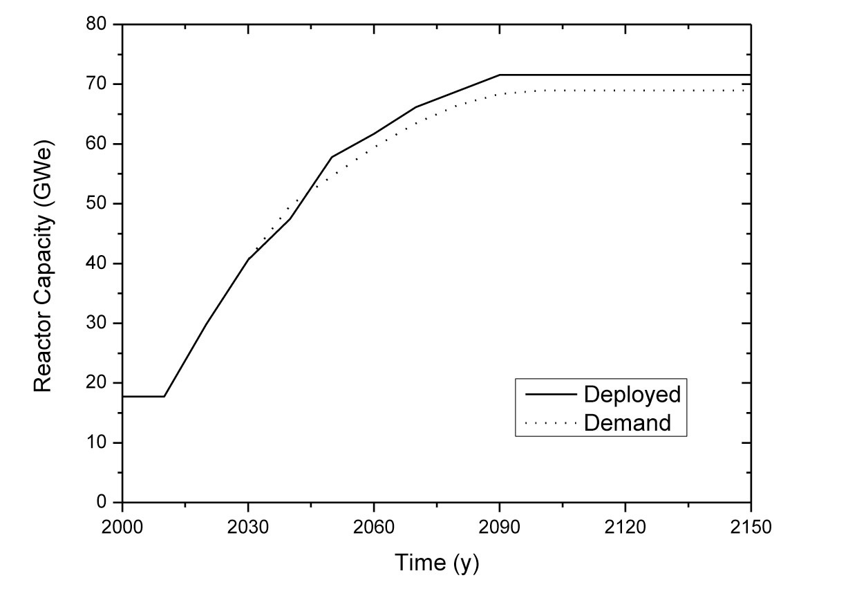
In 2000 the total reactor capacity in Korea was 13.8 GWe. According to the “National Energy Basic Plan”[9], the nuclear capacity will increase to 27.3 GWe with 29 total operating reactors by 2017. Between 2018 and 2030, it is expected that the annual electricity demand growth rate will be 0.95%/yr, and the nuclear power capacity will become 41.3 Gwe, which will provide ~59% of the total
electricity generation. In this calculation, the nuclear growth rate after 2050 is assumed to decrease at the same rate and become 0% in 2100. The lifetime of existing reactors will be extended by 20 yrs for both the pressurized water reactor (PWR) and Canada deuterium uranium (CANDU) reactors. The lifetime of newly constructed reactors will be 60 yrs.
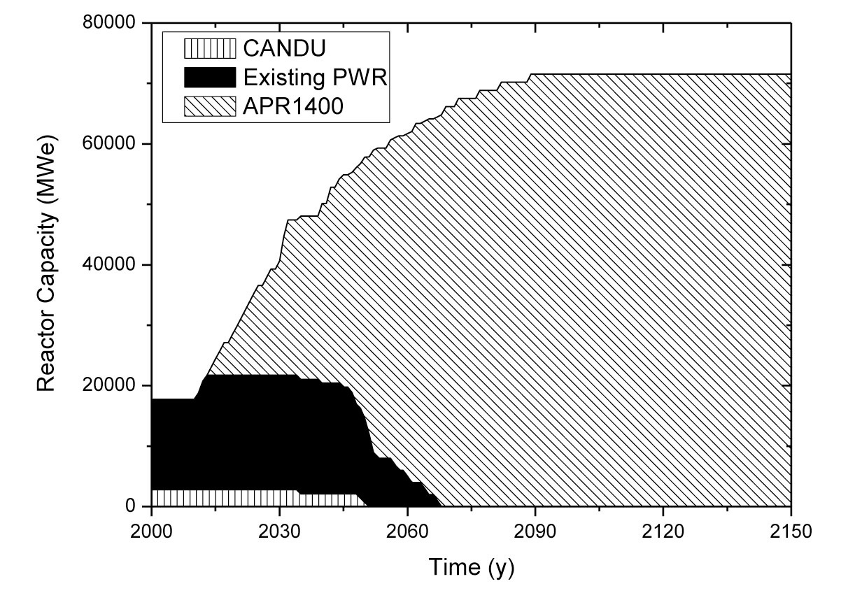
Fig. 1 shows a variation of nuclear power demand and deployed capacity over time. In 2090, both the demand and deployed capacity are expected to be ~70 Gwe, which will be maintained until 2150. Fig. 2 shows the shared capacity of each reactor needed to meet the energy demand. If all CANDU reactors are shutdown, the electricity generation will be dominated by PWRs after 2050. It is also shown that all the existing PWRs are shut down by 2070, consequently advanced pressurized water reactors (APWRs) are dominant after 2070. The number of operating APWRs is expected to be 51 in 2150.
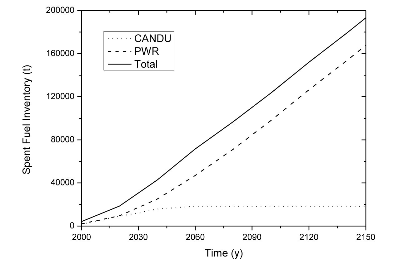
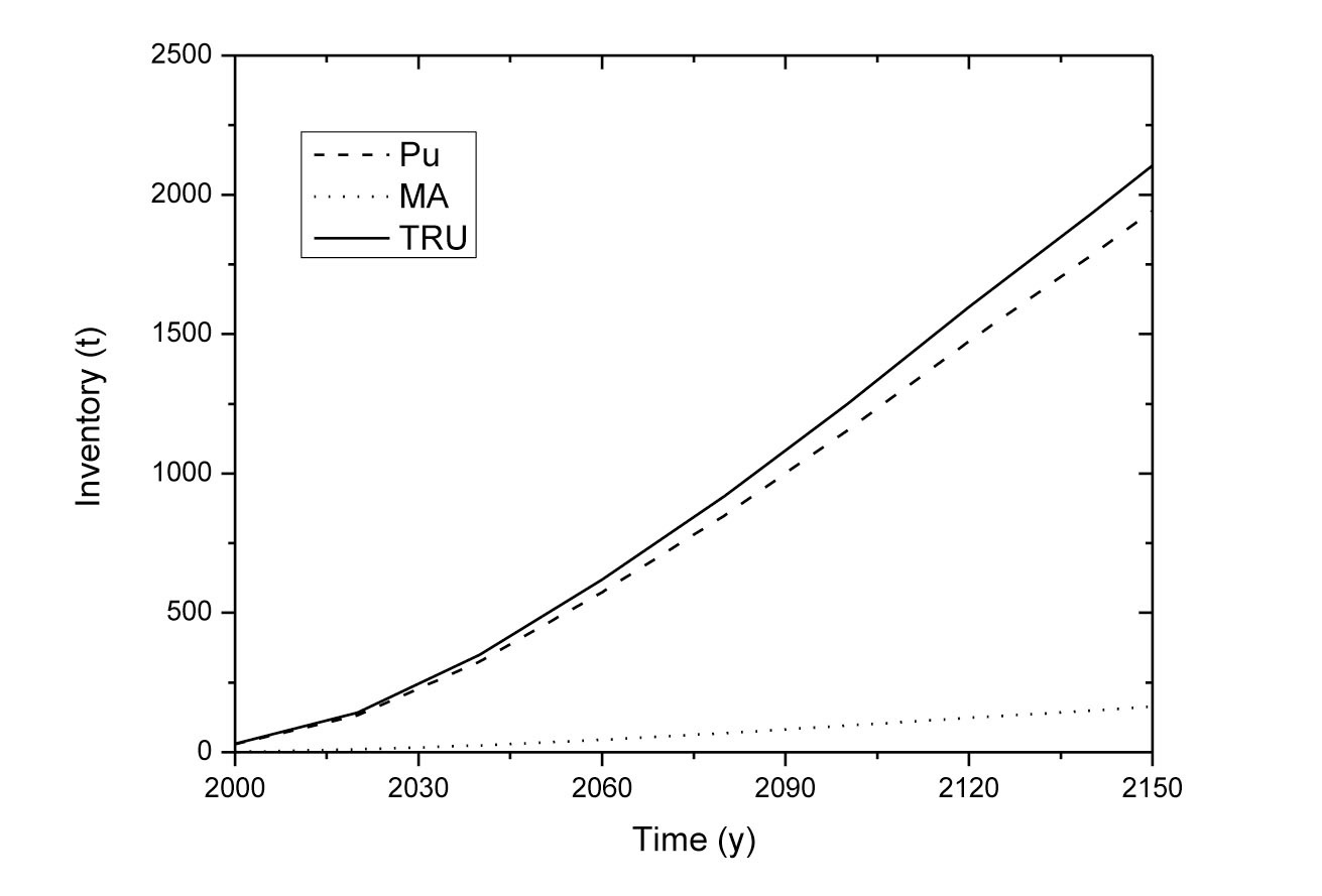
As shown in Fig. 3, the PWR SF inventory continuously increases with time and reaches ~168000 t in 2150. The CANDU SF remains constant at ~18500 t after 2050, as the reactors operations will cease after 2050. Consequently, the total SF is epected to be ~186500 t in 2150. Fig. 4 shows the out-pile TRU inventory. According to the SF inventory, the out-pile inventories of Pu, MA, and TRU
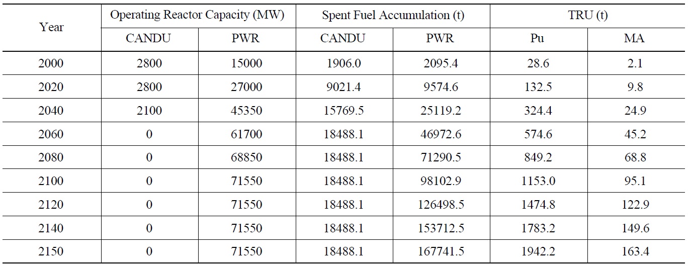
will be 1940 t, 160 t and 2100 t, respectively, by 2150. The fission product (FP) inventory in SF reachs ~8600 t by 2150. Table 1 summarizes the capacity of the operating reactor, SF accumulation, and TRU contents in SF with time.
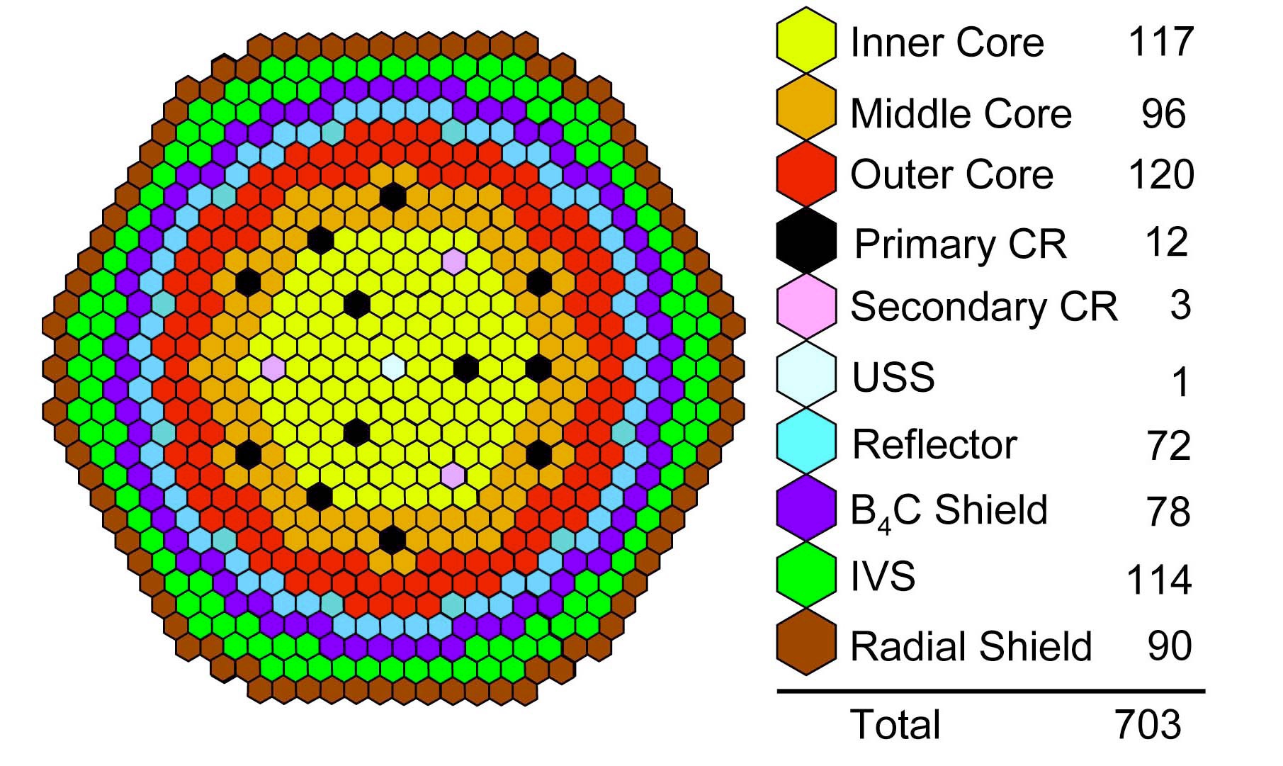
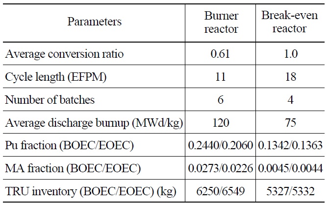
Fig. 5 shows the break-even core, which consists of 117 inner-driver fuel assemblies, 96 middle assemblies, and 120 outer fuel assemblies. The active core height is 94.0 cm, and the equivalent core diameter is 367.03 cm. Each fuel assembly includes 271 fuel pins and has a pin pitch-to diameter (P/D) of 1.167. The outer diameter of the fuel rod is 9.0 mm. The fuel cycle strategy assumed an integral fuel cycle in which almost all the TRU is recycled in the closed fuel cycle. The burner core has small number of fuel assembly and higher fuel enrichment. Table 2 shows the fuel material fraction and inventory change from the beginning of the equilibrium cycle (BOEC) to the end of the equilibrium cycle (EOEC). The FPs including rare earth (RE) elements are assumed to be separated from the TRU in the metal fuel reprocessing.
[Table 1.] Summary of Once-through Cycle Parameters

Summary of Once-through Cycle Parameters
[Table 2.] Fuel Cycle Parameters of Fast Reactor
Fuel Cycle Parameters of Fast Reactor
After one-cycle cooling in In-Vessel Storage (IVS) before the removal from the core, the fuel cycle assumes an 8-month reprocessing, 8-month refabrication, and 2- month storage before being reloaded for an ex-core segment of the fuel cycle. The IVS is used for temporary storage of the irradiated fuel. It was also assumed in the back-end fuel cycle that the pyroprocessing treatment returns 99.9% of the TRU to the core and loses 0.1% to the waste stream. In addition, 5% of the RE fission products are recycled and all other fission products go into the waste stream. Four batch fuel management schemes are used for all three regions of the cores, where one fourth of the fuel inventories in each region is replaced. The burner fast reactor core is different from that of the break-even core, in particular, the TRU enrichment, fuel burnup, and batch scheme for efficient burning of the TRU.
For the deployment fraction of the FR, the capacity of the FR requirement should be determined, as it is limited by the TRU fuel availability. If the reprocessed TRU is compared with the TRU requirement for initial loading and refueling, the deploying FR capcity can be estimated. Of course, the deploying FR capacity may be determined by specific capacity demands. The procdure of the determination of FR capacity is repeated every year. When the FR capacity is determined the difference between the total capacity (Fig. 2) and FR capacity becomes the PWR capacity. In this study, it was assumed that the new FR is deployed from 2040 in the FR fuel cycle. In order to feed the FR, it was also assumed that the PWR SF is reprocessed from 2025 and the FR SF reprocessing begins in 2040. In this study, the CANDU reactor SF is not reprocessed. In the reprocessing, the older SF is reprocessed first. Here, an actual reprocessing capability of industry is not considered, instead, the TRU requirement is used as a constraint of the reprocessing capability. Future reprocessing should take into consideration the capability of the industry.
Recently, the strategy for the management of PWR spent fuel with the use of SFR has been studied [10]. This study, however, has tried to show the FR capacity requirement for burning or reducing the out-pile TRU for both the FR with low and high CR. The FR deployment capacity has been determined as the TRU supply from the PWR SF and FR SF itself. Here, the TRU supply is limited by the reprocessing capacity needed to feed FR. Also, the mixed cases such as deploying the burner first then break-even later or break-even first then burner later, should be investigated. In the calculation, the following four scenarios were analyzed to compare the impacts of FR single or mixing deployments:
- Single burner (BR) deployment: only low CR burner FR is deployed.
- Single break-even (BN) deployment: only high CR break-even FR is deployed.
- BR ? BN mixed deployment: burner FR is deployed first from 2040, then break-even FR is deployed from 2060.
- BN ? BR mixed deployment: break-even FR is deployed first from 2040, then burner FR is deployed from 2060.
3.1 Reactor Deployment and Front-End Parameters
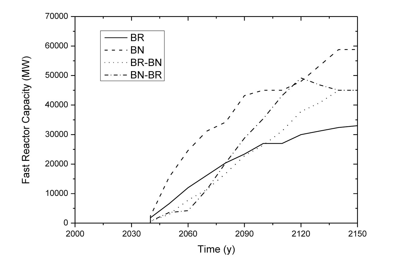
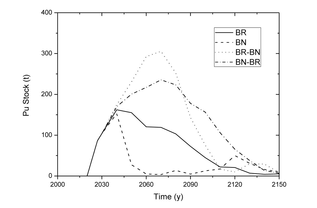
The FR deployment capacities, shown in Fig. 6, are adjusted to match with the nuclear demand so as to minimize the plutonium stock-pile from spent fuel reprocessing as shown in Fig. 7. Here, the deployed FR capacity and Pu stock-piles are different among four scenarios descrived
above. This is the reason for the difference in TRU or Pu requirements of FR with different CR. Also it it is because of the different TRU or Pu feed capacity among the scenarios. The different TRU requirements result in the different Pu stock-pile in each scenario.
For the case of single BR, the FR capacity increases slowly and reaches 33000 MW in 2150. In the single BN case, the FR capacity increases continuously, and becomes 58800 MW, which is the highest value. In the BR-BN mixing case, the FR capacity increases until 2120, then it decreases slightly. The FR capacity of the BN-BR mixing case increases slowly and becomes 45000 MW in 2150.
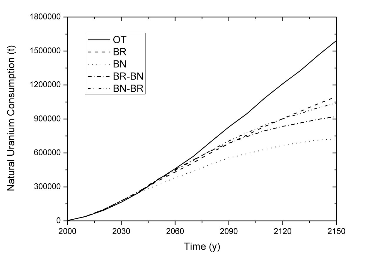
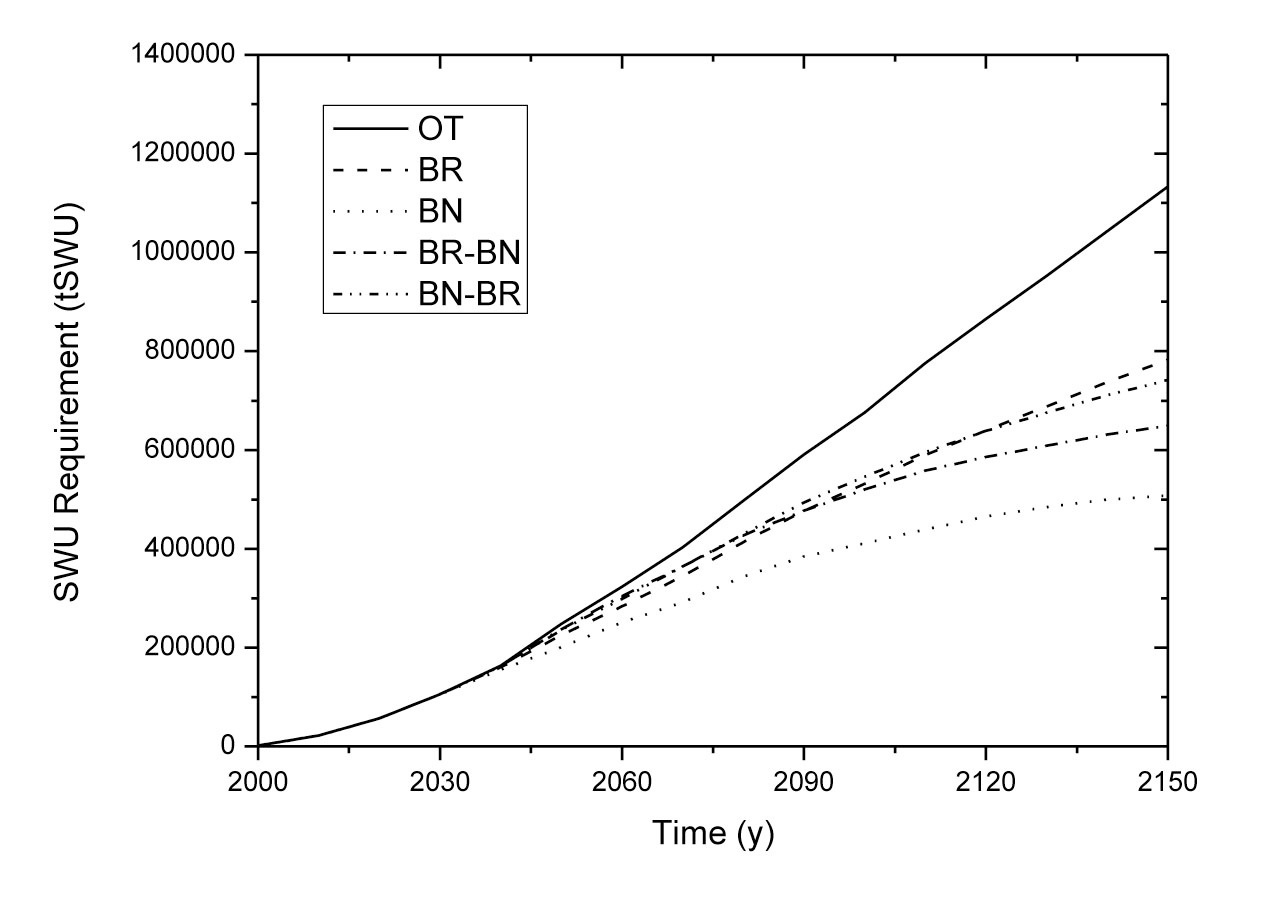
The accumulated natural uranium consumptions are compared in Fig. 8. The uranium consumption decreases as FR deploys since the uranium oxide (UOX) fuel is substituted by the FR fuel. Among the FR cases, the uranium consumption of the single BN case shows the lowest value of 723800 t, which is decreased by ~55% in 2150 as compared with the OT case. For BR-BN and BN-BR mixing cases, the consumptions of natural uranium decrease by ~42% and 35%, respectively. For single BR case, the decreasing of uranium consumption is low since the PWR fraction is higher than other cases. As shown in Fig. 9, the fuel enrichment shows almost the same trends with those
of the natural uranium consumption. These are caused by the decrease of PWR deployments, which are the same for both single and mixed deployment of a FR.
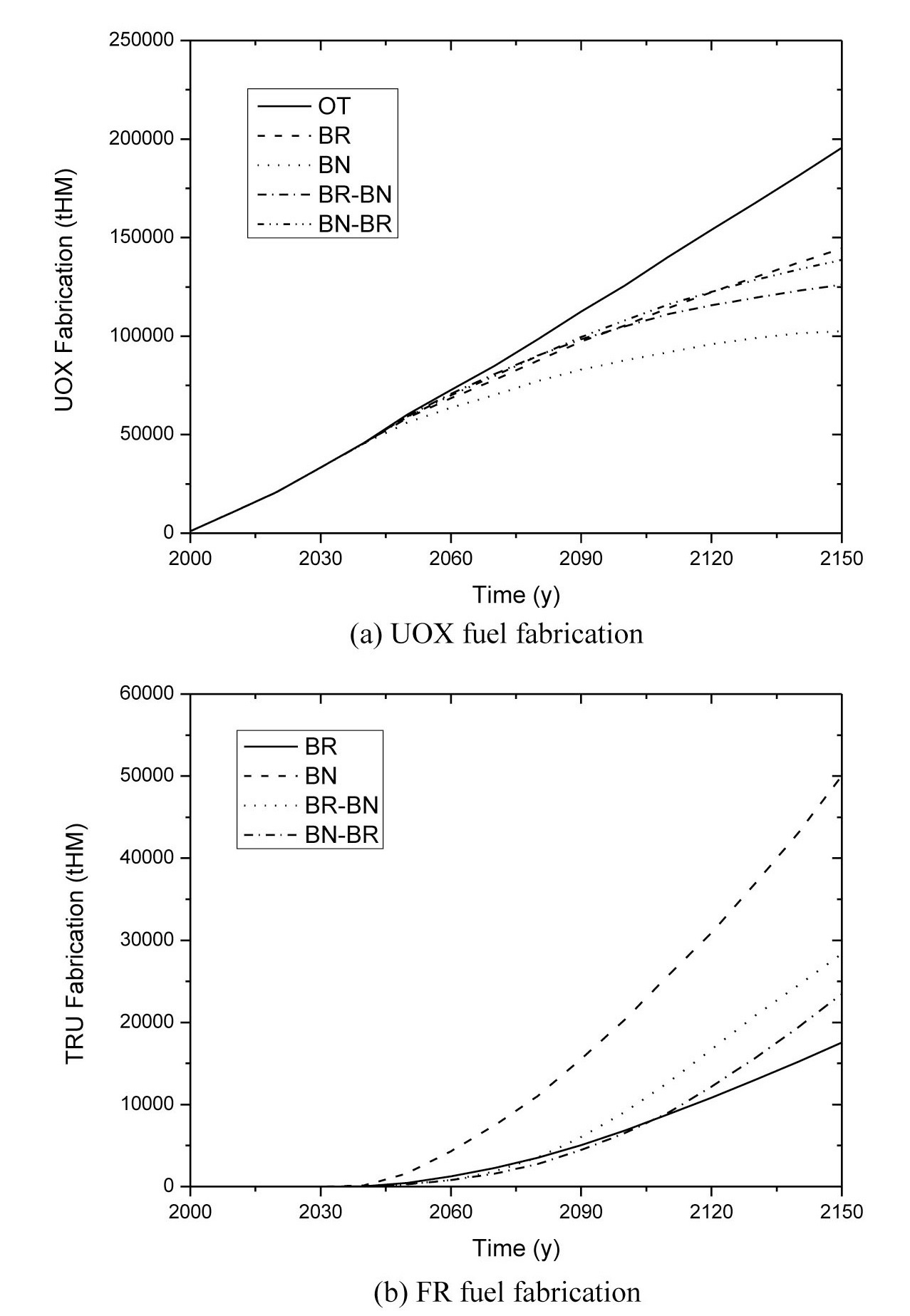
The fuel fabrications are shown in Fig. 10. For single BR and BN cases, the UOX fabrications in 2150 are 144530 t
[Table 3.] Comparison of Total Spent Fuel Inventory

Comparison of Total Spent Fuel Inventory
and 102610 t, which are reduced by 26%, and 48%, respectively, compared with the OT case. The UOX fuel fabrication for BR-BN and BN-BR mixing cases are decreased by ~36% and ~29%, respectively when compared with that of the OT case. The FR fuel fabrication increases with an increase of CR. The FR fuel fabrications in 2150 are 17540 t, 50040 t, 28400 t, and 23460 t, for the BR, BN, BR-BN, and BN-BR cases, respectively.
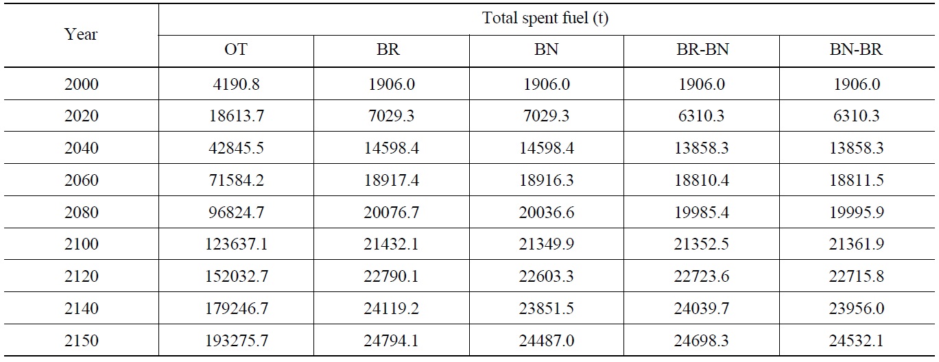
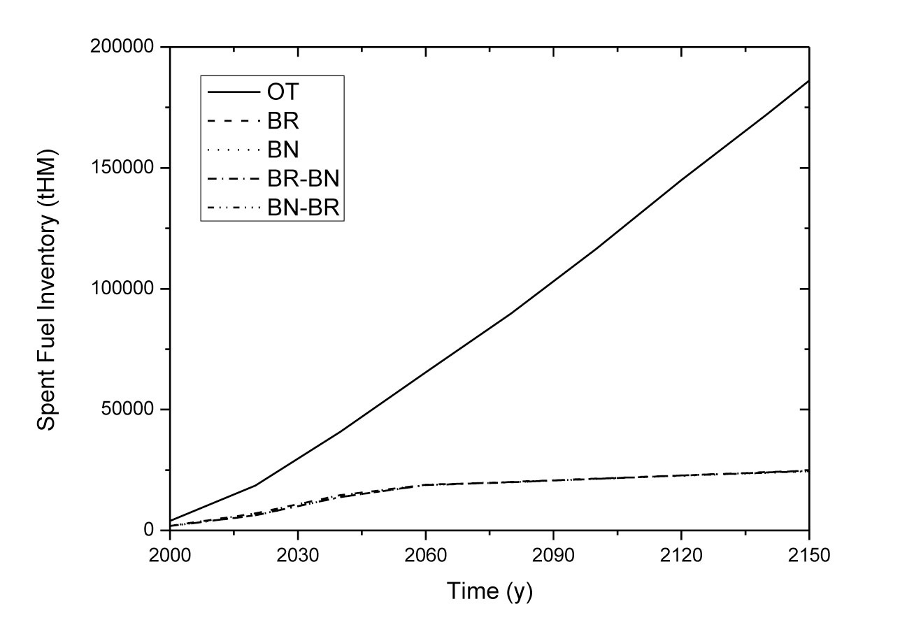
Fig. 11 and Table 3 compare the total amount of the SF between the OT and FR fuel cycles. Here, the total SF includes the HLW (high level waste) which is produced from the reprocessing loss. The amount of the HLW is calculated by the amount of reprocessing multiplied by reprocessing loss. It can be seen that all the FR fuel cycles reduce the total amount of SF by ~87%. This occurs due to the fact that all the PWR SFs should be reprocessed to feed a FR, deployed at the maximum rate, to meet the capacity demand for all cases. In this study, the maximum
FR deployment rate was selected for the maximum reduction of the PWR SF. Here, the reprocessing capacity has been determined based on the TRU requirement for the FR deployment. Therefore, the SF of the FR cases includes
[Table 4.] Comparison of Spent Fuel Reprocessing Amount

Comparison of Spent Fuel Reprocessing Amount
the CANDU SF and PWR SF in the storage pool, interim storage for reprocessing, and reprocessing facilities.
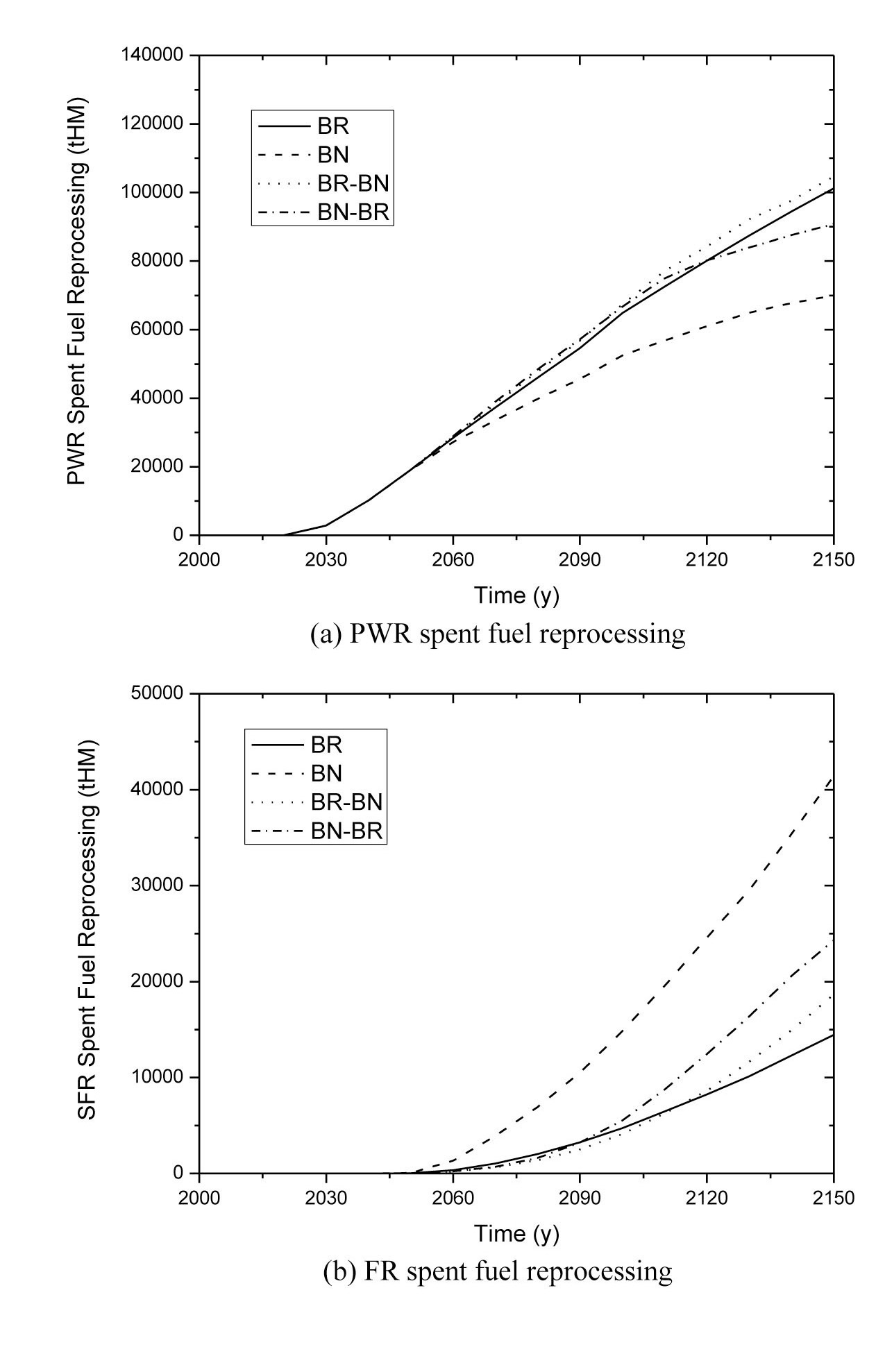
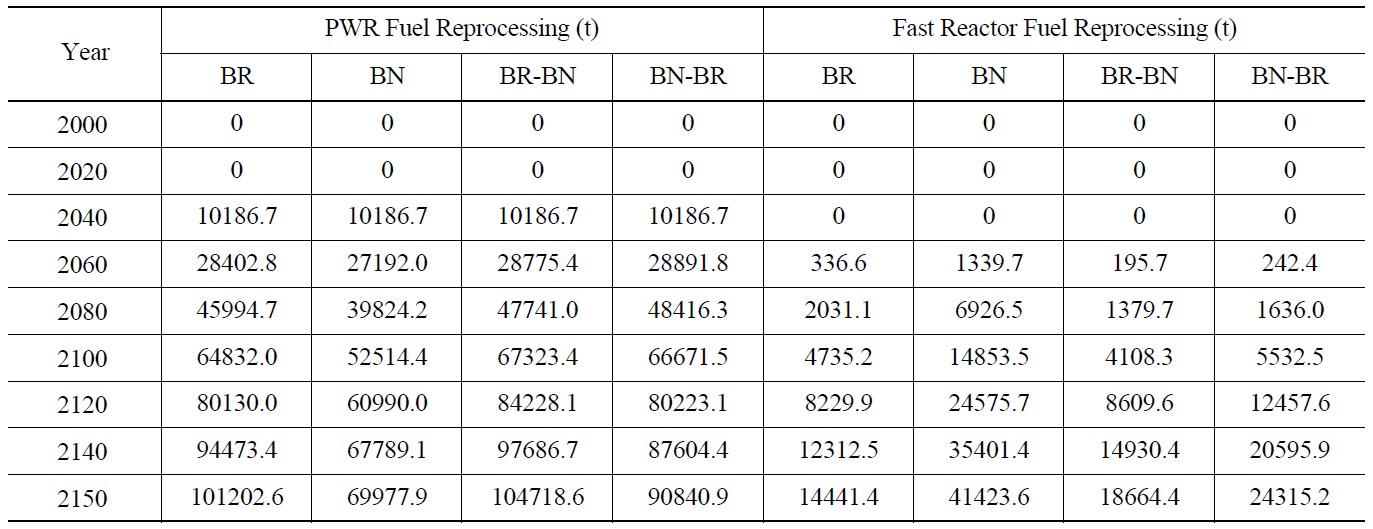
The amount of accumulated SF reprocessing is shown in Fig. 12 and Table 4. As shown in Fig. 12, the amount of PWR SF reprocessing is highest in single BR case. The total PWR reprocessing amounts in 2150 are 101200 t, 69980 t, 104720 t, and 90840 t for the BR, BN, BR-BN, and BN-BR cases, respectively. While, the FR SF reprocessing is highest in the single BN case. The SFR SF reprocessing amoumt in single BR and BN cases are 14440 t, 41420 t, respectively. For the mixing cases, the FR SF reprocessing are 18660 t and 24315 t, respectively for BRBN and BN-BR. Here, it should noted that the FR SF is stored for a short time, and will eventually be reprocessed.
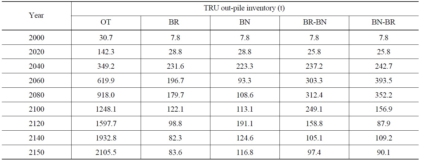
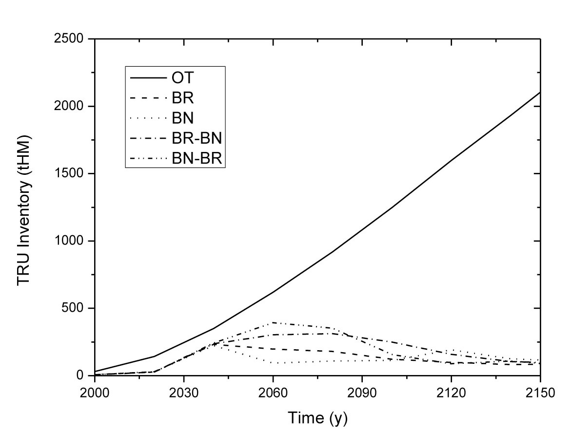
The out-pile TRU inventory includes the TRU in the SF and stock-pile from the reprocessing. The total outpile TRU inventories of each FR case in 2150, shown in Fig.13, are 83.6 t, 116.8 t, 97.4 t, and 90.1 t, respectively. They are reduced by 96%, 94%, 95%, and 96%, respectively, compared to that of the OT. The TRU reduction rate
is very similar in each case, but it should be noted that the single BR deployment scenario shows lower operating FR capacity than other scenarios. Table 5 also summarizes the TRU inventory for each scenario.
In this section, the long-term heat (LTH) load in a repository is analyzed. The LTH is an important parameter determining, among other factors, the packing of waste in the repository [11]. In this study, only the heat load calculation methodology, which has been applied to Yucca Mountain [11], was discussed. In this method, the temperature is limited by 96 ℃ which is caused by the decay heat. The decay heat in the repository performance is the integrated decay heat between the time when the forced ventilation is stopped, and 1500 yrs. In this study, the Yucca Mountain methodology was used since there is no fixed repository strategy and methodology in effect in Korea. The methodology should be changed if the repository is determined to be different from the Yucca Mountain cases.
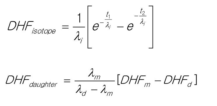
First, the variation of the main isotope inventory change is obtained, and then the LTH is calculated by myltiplying the isotope inventory by the heat load factor (HLF) as,
LTH = Massisotope x HLF, HLF = DHisotope x DHFisotope+DHdaughter xDHFdaughter
where DH= decay heat of isitope or daughter [W/g], DHF=decay heat factor of isotope or daughter [yr].
The DHFisotope and DHFdaughter can be calculated by
[Table 5.] Comparison of TRU Out-pile Inventory

Comparison of TRU Out-pile Inventory
where λi = decay constant of isotope i [1/yr],
λd = decay constant of a daughter of isotope [1/yr],
λm = decay constant of a mother isotope [1/yr],
t1 = starting time of integration [yr],
t2 = termination time of integration [yr].
The cumulative amount of heat generated by the spent fuel and/or high-level waste from disposal to 1500 years after discharge is quantified by integrating the individual isotope decay heat over that period. The total long-term repository heat-load indicator is calculated as the sum of contributions from different isotopes.
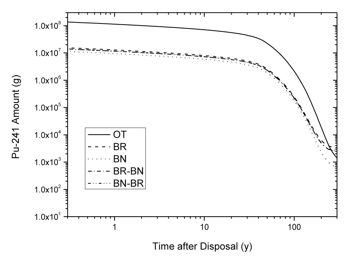
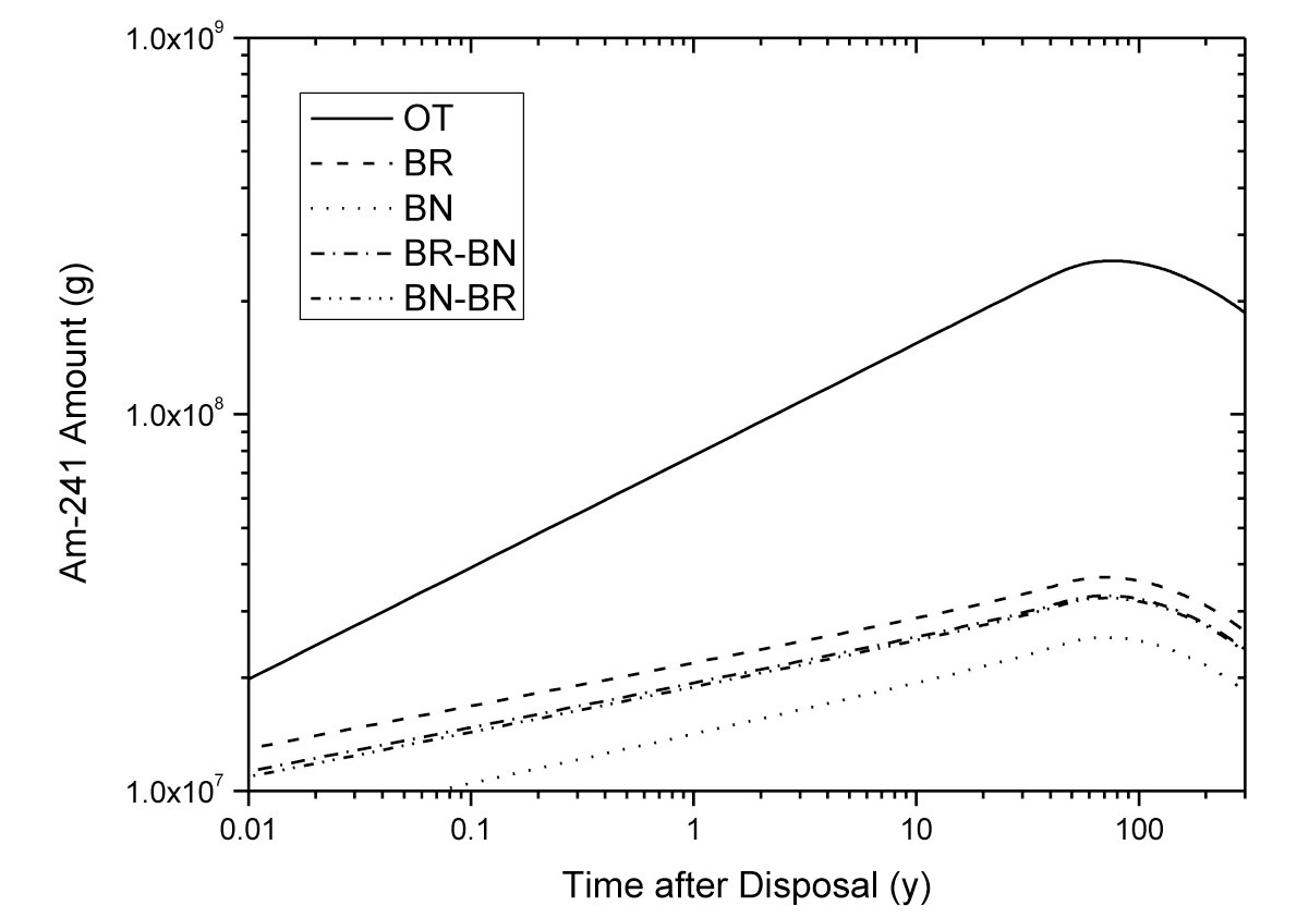
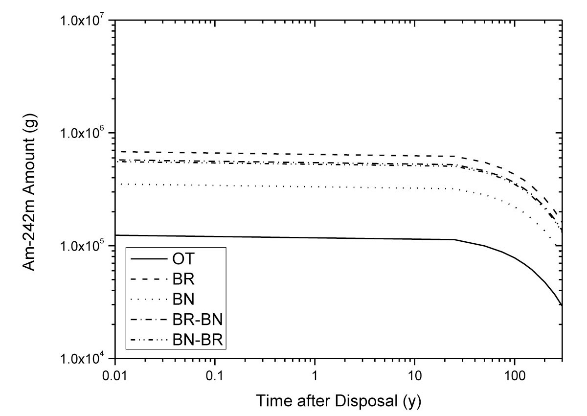
Figs. 14 ? 16 show the main isotope inventory contributing to the heat load after the year 2150. As shown in Fig. 14, the Pu-241 decays very fast, and therefore does not contribute much to the long-term heat load. The Am-241 isotopes, shown in Fig. 15, increase until ~80 yrs after discharge, and then decrease very slowly. The Am-241 is produced by the decay of Pu-241, therefore the Am-241 inventory decreases with anin the CR of a FR since the Pu-241 content is higher in low CR FR. The Am-241
inventory of the BN case is lowest among all the FR cases. The concentration of the Am-242m isotope is compared in Fig. 16. For the FR cases, all the Am-242m isotope concentrations are higher than that of the OT case. This is because the Am-242m is produced by the neutron capture of Am-241 during the irradiation process in the FR. Among the FR cases, the inventory of Am-242m of the single BN case shows the lowest value because of the lowest TRU content.
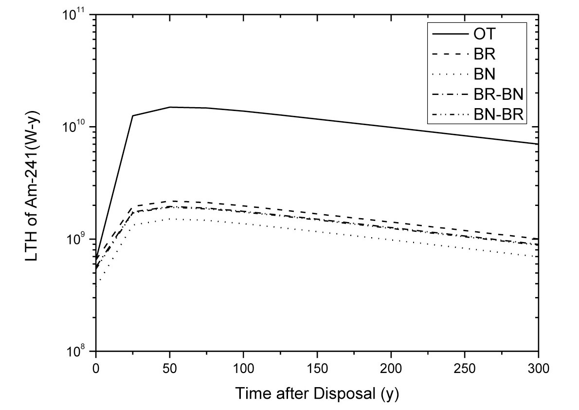
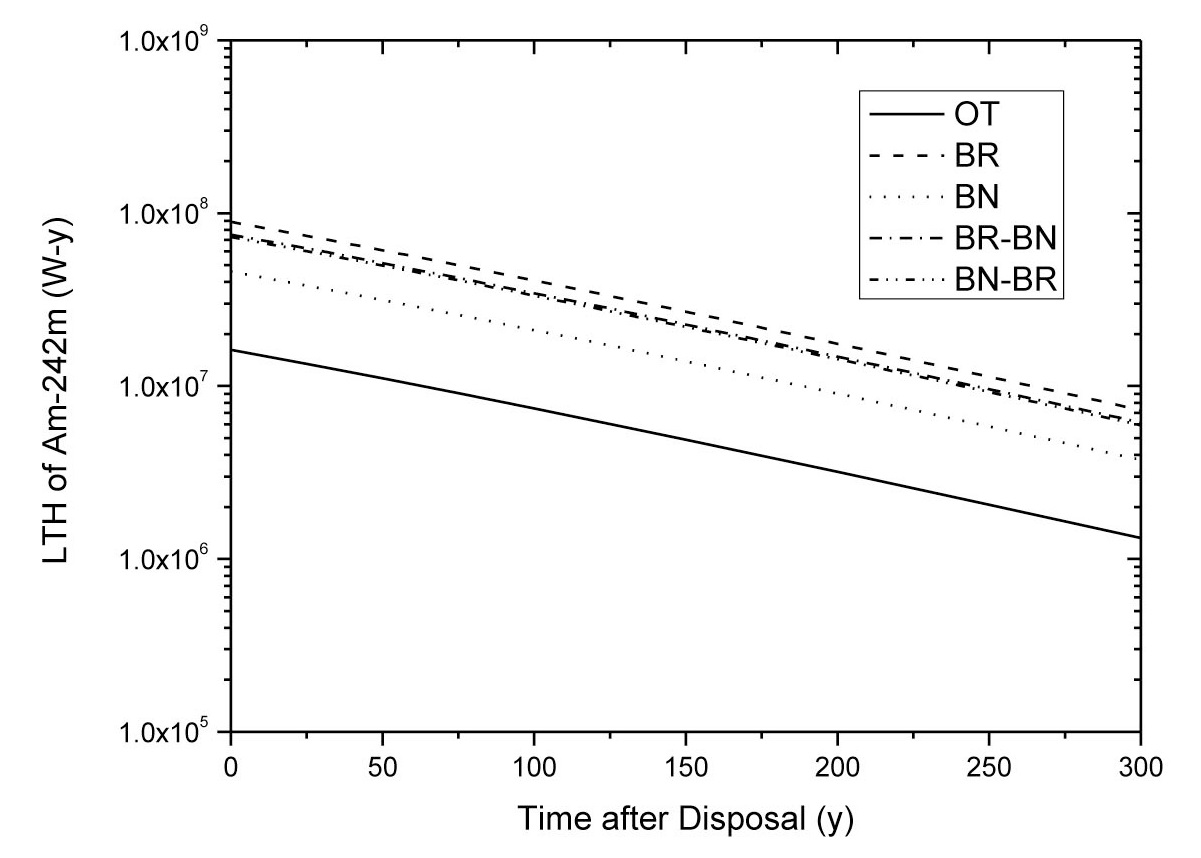
The LTH is found to be contributed mainly by the isotopes of Am-241 and Am-242m, which are shown in Figs. 17 and 18. The LTH of Am-241 are lower for FR cases then the OT case. The LTH of Am-241 decreases with a high CR. The LTH of the OT at 300 yrs after disposal is W-y. The LTH of the BR, BN, BR-BN, and BN-BR cases at 300 yrs after disposal are reduced by 86%, 90%, 87%, and 87%, respectively, compared with that of the OT case. The LTH of Am-242m isotope of all the FR cases are higher than the OT case. These are due to the higher Am-242m isotope concentrations than the OT case. The LTH of Am-242m for the BR, BN, BR-BN,
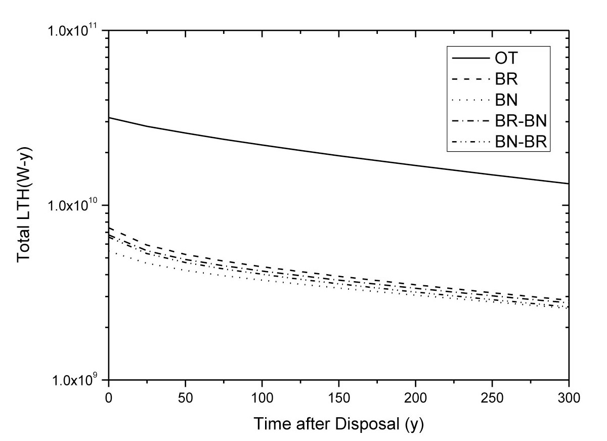
and BN-BR cases at 300 yrs after disposal are 1.03×10⁹, 1.70×10⁹, 1.93×10⁹, and 18.6×10⁹ W-yr, respectively. As shown in Fig.19, the total LTH decreases with an increase
[Table 6.] Comparison of Total LTH after Disposal
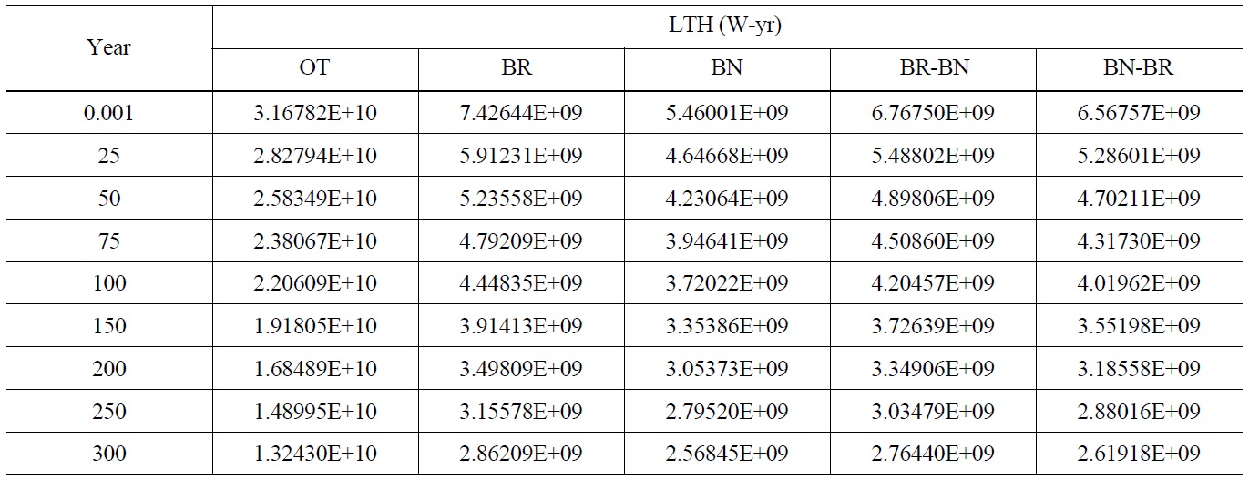
Comparison of Total LTH after Disposal
in CR. At 300 yrs, the total LTH of BR, BN, BR-BN, and BN-BR cases at 300 yrs are 5.87×10⁹, 5.29×10⁹, 5.98×10⁹, and 6.77×10⁹ W-yr, respectively, which are reduced by ~56%, ~60%, ~55%, and ~49% when compared with that of the OT case. From these results, it can be seen that the LTH of the BN-BR is highest among the FR cases. Table 6 also summarizes the LTH for each case.
The results of the FR cycle were compared with those of the once-through cycle. The comparison results for the burner, break-even, burner ? break-even, and break-even ? burner cases can be summarized as follows:
- The total natural uranium requirement and total amount of enrichment in 2150 decrease by 22%, 54%, 30% and 52%, respectively, compared with that of the OT.
- The UOX fuel fabrications in 2150 decrease by 18%, 49%, 25% and 25%, respectively, compared with that of the OT.
- The amount of total SF, if the separated uranium is excluded, is reduced by ~80%, compared to that of the OT.
- The amount of total out-pile TRU can be reduced by 50%, 50%, 48%, and 40%, respectively, compared to that of the OT.
- The most dominant isotope of the LTH is Am-241.
- The total LTH decreases with an increase in CR. At 300 yrs after disposal, the total LTH is reduced by 56%, 60%, 55%, and 50%, respectively, compared with that of the OT.
From the above results, it is shown that the mixing strategies of a FR of low and high CR can effectively reduce the TRU inventory with a low FR capacity, compared with a single break-even deployment. Also, it is known that the mixing scenarios can reduce the TRU inventory with a lower burner capacity than a single CR deployment. In the future, it is recommended to investigate other important fuel cycle parameters such as the economics, and proliferation resistance.