This paper presents a method of improving the performance of a day-ahead 24-h load curve and peak load forecasting. The next-day load curve is forecasted using radial basis function (RBF) neural network models built using the best design parameters. To improve the forecasting accuracy, the load curve forecasted using the RBF network models is corrected by the weighted sum of both the error of the current prediction and the change in the errors between the current and the previous prediction. The optimal weights (called “gains” in the error correction) are identified by differential evolution. The peak load forecasted by the RBF network models is also corrected by combining the load curve outputs of the RBF models by linear addition with 24 coefficients. The optimal coefficients for reducing both the forecasting mean absolute percent error (MAPE) and the sum of errors are also identified using differential evolution. The proposed models are trained and tested using four years of hourly load data obtained from the Korea Power Exchange. Simulation results reveal satisfactory forecasts: 1.230% MAPE for daily peak load and 1.128% MAPE for daily load curve.
Electrical power systems are required to be operated near their full capacity for optimally efficient commercial use. The importance of precise peak load forecasting has increased in the new open access operating environment of electricity supply industries in which companies determine generation, transmission, distribution capacities, and investment as required to reserve generation in real time. To achieve precise short-term load forecasting, various methods including auto-regression, time-series, exponential smoothing, stochastic process, fuzzy logic, and artificial neural networks have been utilized [1-22]. The non-stationarity of the load forecast process, in addition to the complex relationship among variables such as weather, economic situation, holidays, geographical locations, daylight hours, and electric loads, renders artificial neural networks (ANNs) effective. An ANN is a very attractive and commonly applied approach to load forecasting problems, because it has the ability to learn and construct a complex nonlinear mapping based on a set of input and output data. A functional relation between the variables and electrical loads is not required, because the ANN can generate the functional relationship based on learning data. Recently, the ANN has been utilized on its own, or combined with fuzzy logic, to perform load forecasting [1-3,5-9,18-22]. However, there still exist unsatisfactory forecast errors when there are rapid fluctuations in load and temperature.
Radial basis function (RBF) neural networks have been employed for functional approximations in time-series modeling and in pattern classification. Because of their nonlinear approximation properties, RBF neural networks are able to model complex mappings. These networks often require more neurons than standard feed-forward back-propagation networks; however, they can often be designed in a fraction of the time it takes to train back-propagation networks. These networks work best when a large amount of training data is available. RBF neural networks have been employed for functional approximation in time-series modeling because of their nonlinear approximation properties [6,15,19,21,22]. However, these studies did not achieve a precision of less than 1.4% for the mean absolute percent error (MAPE).
This paper presents a method that improves the accuracy of the next-day load curve forecasting. The presented forecasting method uses a hybrid scheme: forecasting is carried out using RBF neural networks with the best design parameters; next, error correction is performed. In an electricity market, the price is set by supply and demand based on day-ahead peak load forecasting. The cumulative forecasting error over the course of a year gives rise to undue profits and losses to buyers and sellers. This error necessitates the settlement of amounts at the end of the year. This problem has not yet been considered in the literature. In this paper, a new day-ahead peak load forecasting method that reduces forecasting errors and their sum over the course of a year is also proposed. Section 2 describes the variables impacting load curve. The average load forecasting errors for holidays and the previous working day are much higher than those for typical working days. To improve the precision of the next-day load forecast, two different RBF neural networks with the best design parameters and their input and output nodes are described. Section 3 describes the error correction for both the load curve and the peak load forecasting. In section 4, performance evaluation is shown using a simulation; the test results show a considerable improvement over previous methods.
2. Load Curve Forecasting Model
2.1 Variables Impacting Load Curve
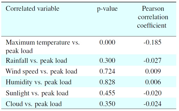
The analysis of daily load and weather data helps to understand the variables that affect load forecasting. The correlation analysis is based on 3 years of data containing the daily peak load, average load, temperature, rain, wind, humidity, sun, and cloud
[Table 1.] Correlation analysis between weather and load

Correlation analysis between weather and load
data. The model results are given in Table 1. In this analysis, the peak load represents the electric load curve, because the peak load has more sharp fluctuations in magnitude. In consideration of the large number of significant correlations (those with p < 0.05) the maximum temperature is shown to be the most influential weather variable affecting the load.
Daily electricity load demand is also influenced by whether a day is a working day, weekend, or holiday. There exists weekly seasonality, but the value of the load scales up and down. The shapes of the load curves on working days and weekends are quite similar [7,10,11,13]. Therefore, the days can be classified into distinct groups, hereinafter called day types, each of which has common characteristics. The day types are normal weekdays (Tuesday?Friday), Monday, Saturday, and Sunday. Monday is different from weekdays because of the pickup load that is seen on Monday mornings. The day types correspond to the days of week in any given month of the year. A holiday has a similar shape to a Sunday; consecutive holidays must be treated separately.
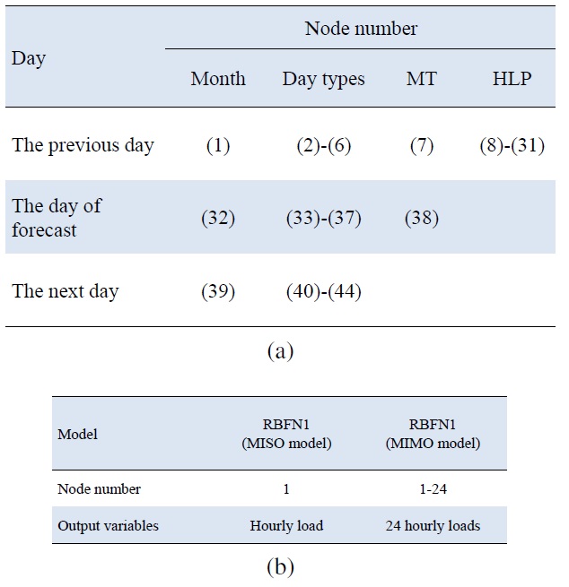
The most important step when building a short-term load forecasting model is correct selection of input variables. In practice, there is no rule that will guarantee correct selection. Selection mainly depends on experience; however, some statistical analysis can be helpful in determining the variables that significantly influence the load. According to the description of months in Section 2.1, the day types and the maximum temperature should be included in the input variables of the RBF neural networks. It is known that the load at a given hour is dependent not only upon the previous hour but also upon the load at the same hour on the previous day. Hence, the 24-h load profile for the previous day of forecast is also included in the input variables. The day types are defined by five binary digits, in which each digit is either 0 or 1, depending on whether the day is Monday, Tuesday?Friday, Saturday, or Sunday, and a holiday or not. The day types for the next day’s forecast are also utilized as the input variables so as to handle consecutive holidays and the working day before them.
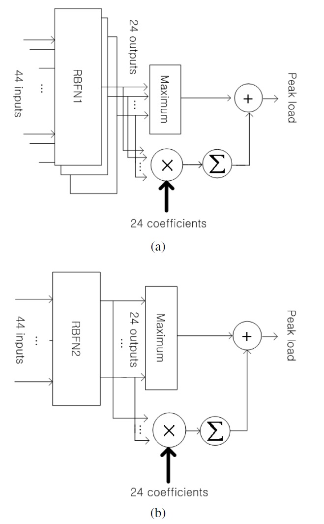
Two types RBF neural network models are used for 24-hahead load forecasting: 24 multi-input single output (MISO) models and multi-input multi-output (MIMO) models, hereinafter called radial basis function neural network (RBFN)1 and RBFN2, respectively. These models use the same 44 input nodes shown in Figure 1; their 24 output nodes are composed of the forecasted 24 hourly load curves. The maximum value of the load curve becomes the forecasted daily peak load. Neural networks applied in traditional short-term forecasting use whole similar days’ data to learn trends of similarity. The learning of all of the similar days’ data is complex and results in relatively large errors. Recently, similar day-based neural network methods in which only the similar day load selected by similarity analysis is used as the input load have been applied [5,8,20]. However, these networks do not have satisfactory performance, in spite of the additional computational load.
In this paper, the RBFN models utilize the entire load dataset. The models were built and tested using the MATLAB function “newrb.” The function iteratively creates a radial basis network, one neuron at a time, until the maximum number of neurons has been reached. It is important that the spread parameter be large enough that the neurons of the transfer functions respond to overlapping regions of the input space, but not so large that the neurons fail to respond in the same manner. Therefore, the maximum number of neurons and the spread for the network are the design parameters to be determined. To reduce the forecasting error, the best design parameters for the RBFN models are selected using grid searches.
3. Load Forecasting with Error Correction
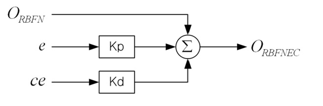
The proposed error correction method attempts to minimize the forecasting error by implementing two error compensation strategies: the proportional and the derivative, as shown in Figure 2. Proportional compensation makes a change to the forecasting value that is proportional to the current error value.
The error value is then calculated as the difference between the real electric load and its forecasted value. Proportional compensation is obtained by multiplying the error by a constant called the proportional gain. A high proportional gain results in a large change in the forecasting value for a given change in the error. By contrast, a small gain results in a small response to a large input error and less-sensitive compensation. The change rate of the errors is calculated by subtracting the current day’s forecasting error from the previous day’s forecasting error. Derivative compensation is obtained by multiplying the rate of change by a constant called the derivative gain. The derivative compensation slows the rate of change of the forecasting value.
The error correction shown in Eq. (3) is carried out by adding the error compensation term of Eq. (1) to the value forecasted by the RBFN models.

Here, ec is the error compensation term, error
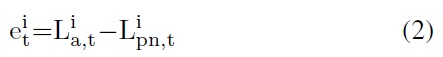

is the value forecasted by the RBFN models, and

is the actual load value.
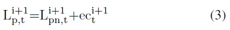

is the value forecasted with the error correction.
Since the magnitudes of the gains influence on the performance of the forecasting the optimal gains minimizing the forecasting error have to be determined. The gains that produce the best error correction are searched using differential evolution (DE) [23]. DE is a method that optimizes a problem by trying to improve a candidate solution iteratively, based on a given measure of quality. DE is used for multidimensional realvalued functions but does not use the gradient of the problem being optimized. DE optimizes a problem by maintaining a population of candidate solutions and creating new candidate solutions (by combining existing ones according to its simple formulae), and then keeping whichever candidate solution has the best fitness for the optimization problem at hand. In this way, the optimization problem is treated as a black box that merely provides a measure of quality for a given candidate solution; the gradient is, therefore, not needed. As the measure of quality to evaluate the candidate solution, the MAPE of Eq. (4) is utilized. DE is carried out to identify the gains that will minimize the MAPE.
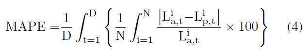
and
are the actual and forecast values of the load curve, respectively, N is the number of the hours of the day i.e., N = 24, and D is the number of the forecasted days.
An electricity market is a system for effecting purchases, through bids to buy; sales, through offers to sell; and short-term trades. To set the price bids and offers, supply and demand based on day-ahead peak load forecasting is used. The forecasting error gives rise to undue profits and losses to buyers and sellers. This requires the settlement of amounts at the end of the year. Therefore, reducing the sum of the forecasting errors over a year is no less important than minimizing the individual errors.
The peak load is the maximum value of the daily load curve forecasted by the RBFN models described in section 2. To forecast the daily peak load more precisely, a new method for correcting the peak load is presented. This method attempts to reduce both the MAPE, as in Eq. (5), and the sum of errors (SE), as in Eq. (6). Correction is accomplished by combining the 24-h load curve outputs linearly with 24 coefficients to the peak load, as shown in Figure 3. The optimal coefficients that reduce the error function, as in Eq. (7), are searched using DE.
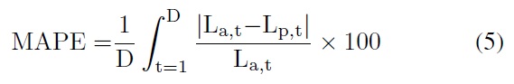
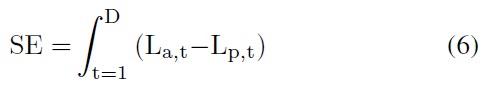
La,t and Lp,t of (5) and (6) are the actual and forecast values of the peak load, respectively. D is the number of the forecasted days.

Using DE, the best solution, which corresponds to the 24 optimal coefficients, can be identified. As the measure of fitness for evaluating the candidate solution, the error function in (7) is utilized.
The performance of the proposed method is evaluated on the basis of a four-year dataset provided by the Korea Power Exchange (KPX). Three-year data from January 2005 to December 2007 are used for learning the RBFN models and for identifying the error correction gains. Load curve forecasting is performed for one year of data from 2008 so as to evaluate the accuracy of the learned models and the error correction. The best design parameters for the RBFN models, as shown in Table 2, are found using grid searches, which are performed over 60 to 95 neurons and 1 to 15 spread values with the grid point steps of 1 and 0.1, respectively.
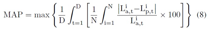
Using the day types for the next day of forecast for the input variables decreases the error considerably, as shown in Table 3. The forecast deviations from the actual values are calculated using Eq. (4), and the maximum absolute percent error (MAP) is calculated using Eq. (8).
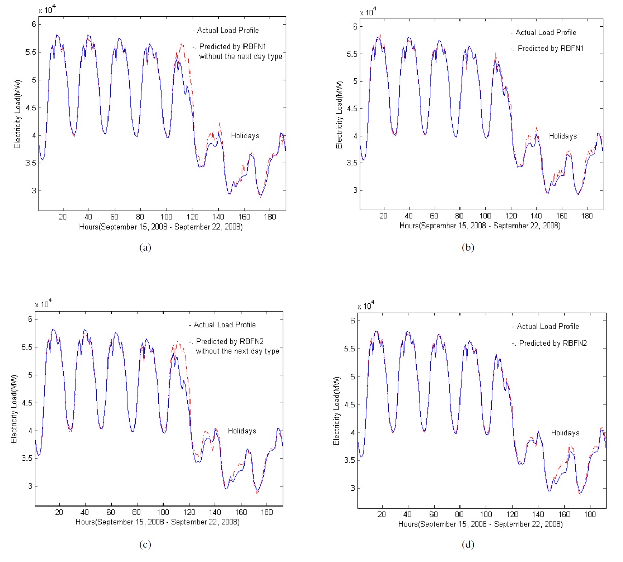
The minimum (5.8%) and maximum (39.0%) errors for RBFN1, and the minimum (5.8%) and maximum (10.2%) errors for RBFN2 are reduced. Figure 4 shows the forecasted result for 8 days from Saturday to the next Monday including special
[Table 2.] The design parameters for the RBFN models
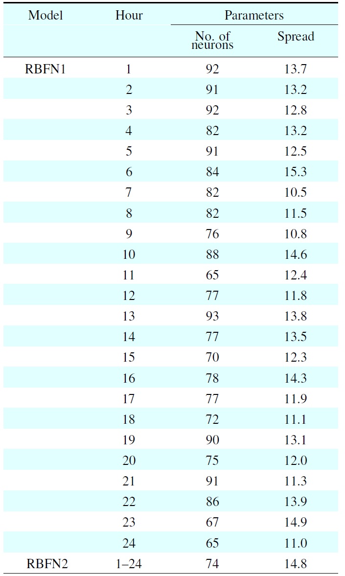
The design parameters for the RBFN models
holidays. Our results indicate that the use of the next day type is effective in predicting the load curve for the working day before the holidays.
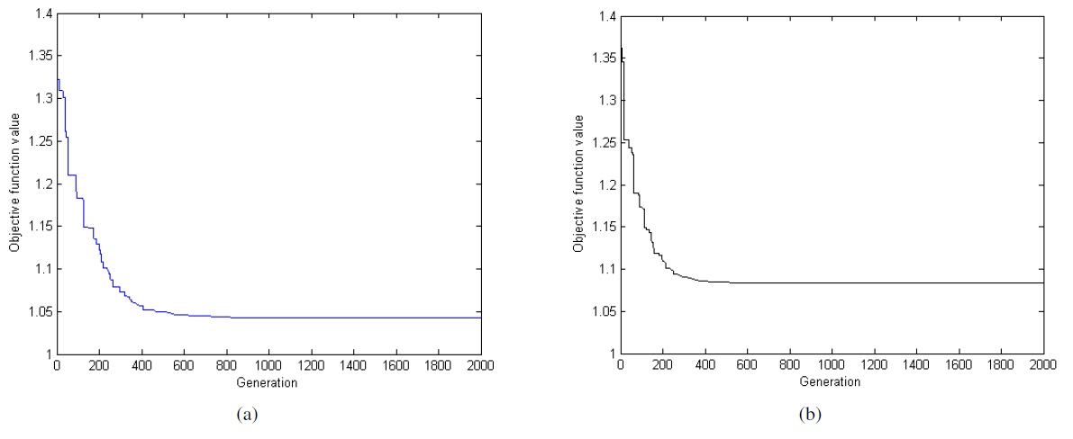
For the best error correction, 48 gains of 24 kp’s and 24 kd’s minimizing (4) are searched using DE. The following control parameters for differential evolution are used: population size = 20, maximum generation number = 2000, differential amplification factor = 0.5, and crossover rate = 0.5.
In the evolutionary process, the objective function values of Eq. (4) decrease, as shown in Figure 5. The identified gains for the best error correction are shown in Table 4. To demonstrate the effectiveness of the proposed method, we applied it
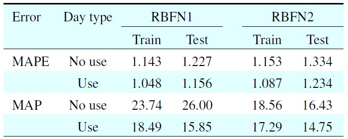
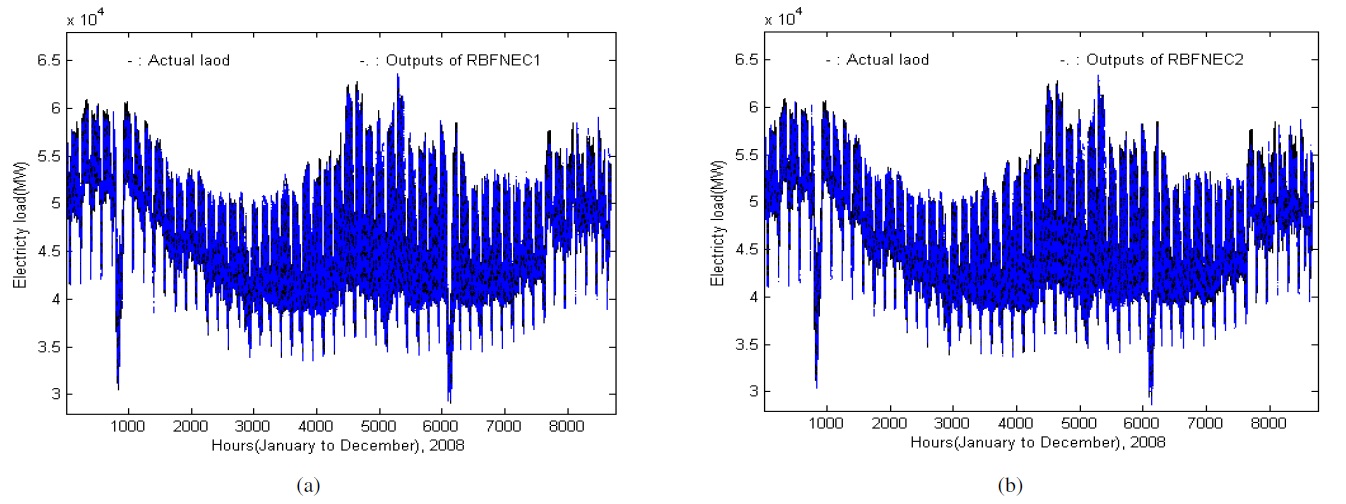
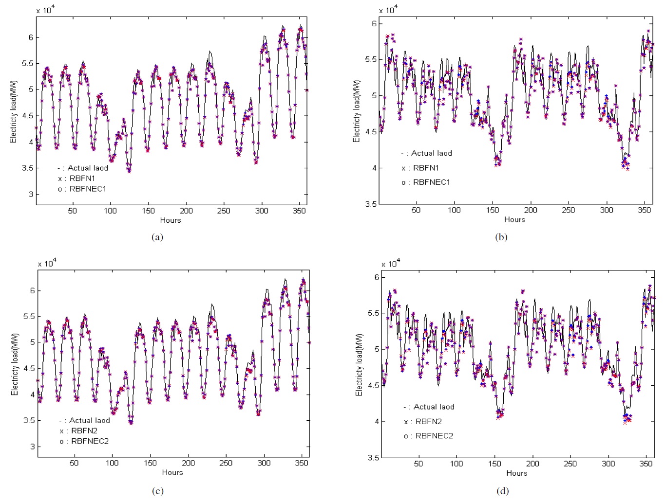
to a section of 2008 in which all seasons under changing conditions are considered. 24-h ahead load curve forecasts from RBFNEC1 (RBFN1 with error correction) and RBFNEC2 (RB FN2 with error correction) are shown in Figure 6. From among the results, those for two weeks each in summer and winter are shown in Figure 7. As shown in Table 5, error correction reduced the MAPE of 1.156 for RBFN1 to 1.128 (by 2.42%) and the MAPE1 of 1.234 for RBFN2 to 1.196 (by 3.08%). The error correction contributes to reducing the comparatively large MAPE of the RBFN models.
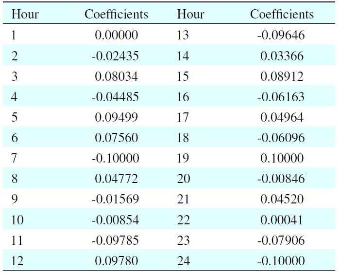
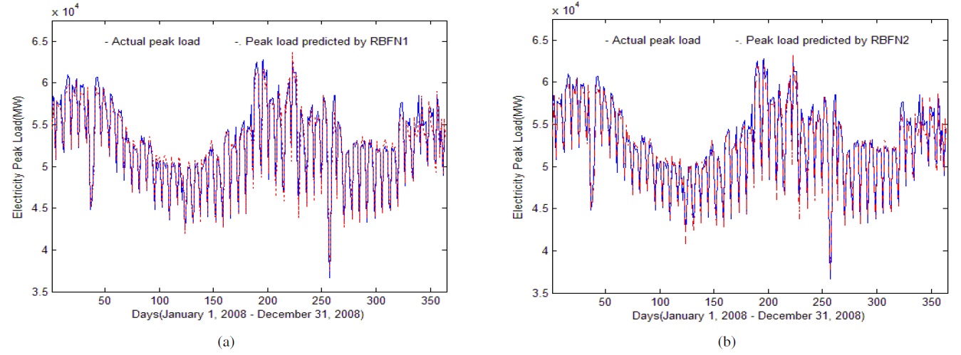
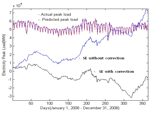
In the evolutionary search of 24 coefficients that minimizes Eq. (6), the following DE control parameters are used: population size = 12, maximum generation number = 500, differential amplification factor = 0.5, and crossover rate = 0.5. The optimal coefficients identified by the search are given in Table 6. The peak load forecasting errors are given in Table 7, which shows that the correction reduces both the MAPE and SE. The peak load forecasting results from RBFN1 and RBFN2 are shown in Figure 8. Figure 9 shows that the correction reduces the SE by less than one-ninth at the end of the test year.
[Table 3.] Effect of day type on the next day’s forecast

Effect of day type on the next day’s forecast
This paper presents a day-ahead load curve forecasting method that combines the RBFN model with an error correction method. To distinguish a similar day’s load from the remainder of the data, the RBFN model includes the day type for the next day in the forecast, in addition to those of the previous and the day of forecast as its input variables. The RBFN model is designed on the basis of the optimal number of neurons and spread, which are found using grid searches. The proportional and the derivative gains for the best error correction are identified by differential evolution. The peak load obtained from the RBFN model is also corrected by adding linear combination of the 24-h load curve outputs and 24 coefficients to itself. The coefficients are optimized to minimize both the MAPE and the SE errors through DE. The experimental results show that the RBFN model combined with the error correction method produces accurate load curves and peak load forecasts and is robust to weather and seasonal variations. The proposed error
[Table 4.] Optimal gains for the error correction
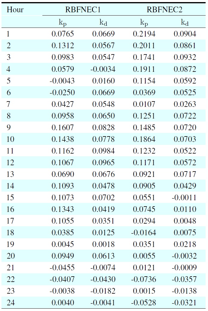
Optimal gains for the error correction
[Table 5.] Error correction results
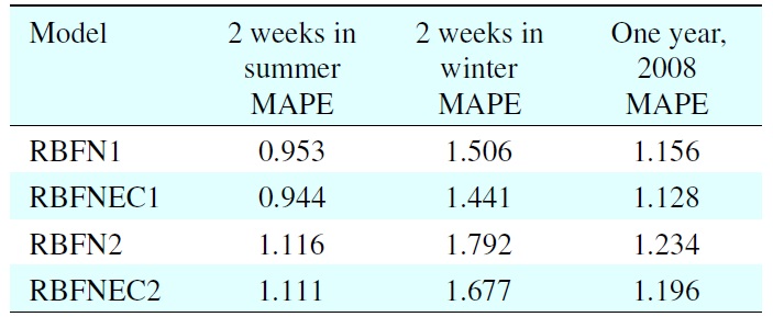
Error correction results
[Table 6.] Identified optimal coefficients

Identified optimal coefficients
correction method is amenable to real-time implementation with hourly or daily gains to adapt and update based on the changing conditions.
No potential conflict of interest relevant to this article was reported.
[Table 7.] Peak load forecasting errors
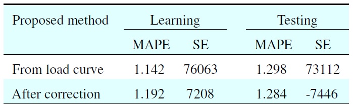
Peak load forecasting errors