Motor imagery classification in electroencephalography (EEG)-based brain?computer interface (BCI) systems is an important research area. To simplify the complexity of the classification, selected power bands and electrode channels have been widely used to extract and select features from raw EEG signals, but there is still a loss in classification accuracy in the stateof- the-art approaches. To solve this problem, we propose a discriminative feature extraction algorithm based on power bands with principle component analysis (PCA). First, the raw EEG signals from the motor cortex area were filtered using a bandpass filter with μ and β bands. This research considered the power bands within a 0.4 second epoch to select the optimal feature space region. Next, the total feature dimensions were reduced by PCA and transformed into a final feature vector set. The selected features were classified by applying a support vector machine (SVM). The proposed method was compared with a state-of-art power band feature and shown to improve classification accuracy.
A brain?computer interface (BCI) is a non-muscular communication system that people can use to directly communicate their intentions from their brains to the environment [1,2]. The BCI system attaches a function to brain signals, thereby creating a new communication channel between the brain and external devices. This communication method is partially focused on the brain signal features extracted by the BCI system for device control and provides mutual interaction between the user and the system. Using different sensors and brain signals, many studies over the past two decades have evaluated the possibility that BCI systems could provide new augmentative technology without muscle control [3-8]. BCI systems have measured specific features of brain activity and translated them into device control commands. For example, an arbitrary limb movement changes the brain activity, such as electroencephalography (EEG), in the related cortex. In fact, even preparing to move and imaging a movement changes the so-called sensory rhythms. We can record
The decrease of oscillatory activity in a specific frequency band is called event-related desynchronization (ERD). Correspondingly, the increase of oscillatory activity in a specific frequency band is called event-related synchronization (ERS). The ERD/ERS patterns can be volitionally produced by motor imagery, which is the process of imagining the movement of a limb without actual movement [9]. In general, EEGs are recorded over primary sensorimotor cortical areas that often display 8?12 Hz (
This paper is organized as follows. In Section 2, we briefly describe related works for discriminant power feature selection, such as Laplacian spatial filter and principal component analysis (PCA). We explain the discriminant power feature selection method and motor imagery pattern classification method in Section 3. A motor imagery EEG classification experiment is introduced and the results are discussed in Section 4. Finally, in Section 5, we conclude this paper and suggest future works for improving our work.
General EEG signal analysis in BCI systems consists of three major parts: preprocessing, feature extraction, and classification of the EEG mental tasks. In this study, the proposed method focuses on the feature extraction step. The initial procedure in feature extraction employs a spatial filter. The purpose of using a spatial filter is to reduce the effect of spatial blurring from the raw signals. Spatial blurring is an effect of the distance between the sensor and the signal sources in the brain and is caused by the inhomogeneities of the tissues between the brain areas. Several spatial filtering approaches have attempted to increase system fidelity. The most typical realization is a Laplacian filter, which consists of discretized approximations of the second-order spatial derivative of the two-dimensional Gaussian distribution on the scalp surface. A Laplacian filter attempts to invert the process that blurs the brain activities detected on the scalp. The approximations can be further simplified. For example, at each time point
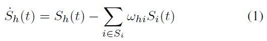
Eq. (1) shows a description of the Laplacian filter.
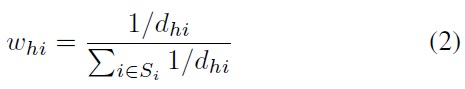
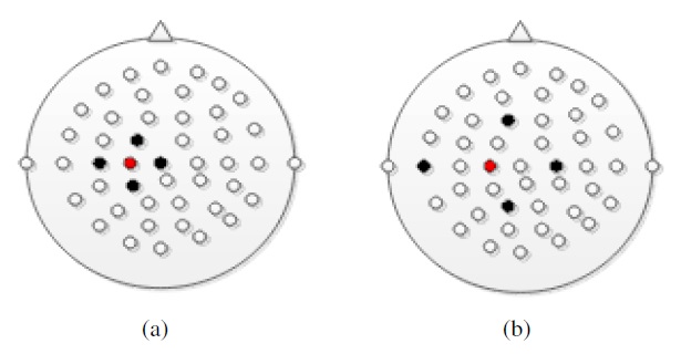
The main purpose of the spatial filter is to derive a more faithful representation of the sources within the brain and/or to remove the influence of the reference electrode from the signal. The influence is sensitive to the Laplacian mapping size as shown in Figure 1. In Figure 1 (a) and (b), the red and black dots indicate the location of the reference electrode and its spatial filter, respectively.
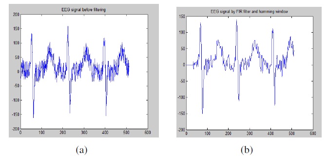
2.2 FIR Filter and Hamming Window
As described earlier, motor imagery has been shown to produce changes in the
Figure 2 (a) shows raw EEG signals without the FIR filtering and Hamming window processing, while Figure 2 (b) shows the result of a filtered EEG signal by FIR filter.
The power bands are calculated from all electrodes of the extracted EEG with an epoch time of 1 second and a 0.5 second
delay from each epoch out of 4 second, during which human subjects start imagining a motor task (such as left/right hand or foot movement) and then finish it. We used 20% of the dataset as the testing set. The remaining 64% and 16% of the dataset were alternately used for training and validation.
2.3 Principal Component Analysis (PCA)
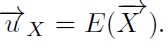
Real-world data is often noisy because various signals from different perspectives are recorded and information is hidden in a few dimensions. PCA is a classical statistical method used to re-express the noisy data in a different framework. This linear transform has been widely used in data analysis and compression. PCA is based on the statistical representation of a random variable. Suppose that we have a random vector population,

where

and the population mean is denoted by
Mean subtraction from each data dimension is necessary for performing PCA to ensure that the first principal component describes the direction of maximum variance. If mean subtraction is not performed, the first principal component might instead correspond more or less to the mean of the data. A mean of zero is needed to find a basis that minimizes the mean square error (MSE) of the approximation of the data. The singular value decomposition (SVD) of
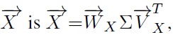
where the

is a matrix of the eigenvectors of the covariance matrix
matrix ∑ is an

is a matrix of the eigenvectors of the covariance matrix
Under this condition, the principal component

of a dataset

can be defined as
With the first

as shown in Eq. (4):
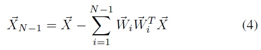
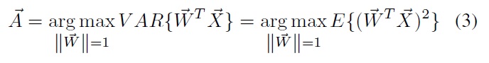
We can achieve our goal of decorrelating the original dataset and reducing its dimension. Many methods exist for solving eigenvalues and corresponding eigenvectors, which is a nontrivial task. By ordering the eigenvectors in a descending order, we can create an ordered orthogonal basis with the first eigenvector (corresponding to the largest eigenvalue) having the direction of the largest variance of the data. In this way, we can find directions in which the dataset has the most significant amount among the multiple dimensions.
Our goal is to find a new matrix

which is a dimensionalityreduced random variable dataset, such that the covariance matrix
is a diagonal matrix, and each successive dimension in

is rank-ordered according to variance from the

Now, PCA allows us to find

It assumes an orthogonal matrix that acts as a transition matrix or function, as in
3. Discriminant Power Feature Selection Using PCA and Classification Using Support Vector Machine
3.1 Discriminant Power Feature Selection using PCA
In this study, the motor imagery EEG signals are represented as
which were segmented from 1 second before the cue onset and 4 seconds after the cue onset of raw EEG signals for a total 5 seconds long time interval from 59 channels. The raw signals were sampled at 100 Hz, and they were spatially bandpassfiltered at 7?15 Hz and 18?22 Hz. We calculated a set of data that consists of a sample mean of
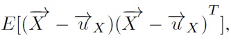
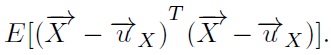
and a covariance matrix of

for each motor imagery state: {left/right hand, foot movement}. For PCA to work properly, we subtracted

from each data dimension in

This produced a dataset with a mean that is equal to zero.
Let
be a transition matrix that consists of eigenvectors of the covariance matrix as the row vectors. It is applied to reduce the dimensionality of
as shown in
Our goal is to find a matrix

The rows of
are the principal components of
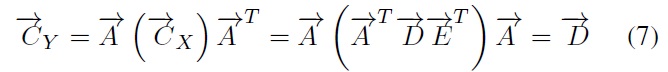
Now, combining all the above information, we have
If

is orthogonally diagonalizable, it can be applied to the SVD such that
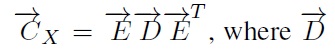
is a diagonal matrix and

is an orthogonal eigenvector that is diagonal to the symmetric matrix

Then, the
is the
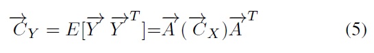
Therefore, we can rewrite Eq. (5) as
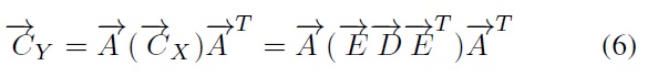
In this case,
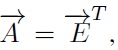
so that
By setting the principal components
equal to the eigenvectors

we can achieve dimensionality reduction.
The original vector
was projected on the coordinate axes defined by the orthogonal basis. It was then reconstructed by a linear combination of the orthogonal basis vectors. Instead of using all the eigenvectors of the covariance matrix, we may represent the data in terms of only a few basis vectors of the orthogonal basis. If we denote the matrix having

we can create a similar transformation. This means that we project the original data vector on the coordinate axes having dimension
In this study, PCA was applied to reduce the dimensionality of the transformation matrix of the training set to
which is used to calculate the final feature using Eq. (8), where the transposed matrix of

has a dimension of
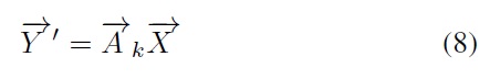
The output feature

is reduced to the
3.2 Classification of Discriminant Power Feature Using SVM
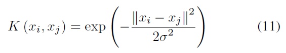
The classification of the discriminant power feature is the most important step in analyzing motor imagery EEG signals. After we selected the optimal features as described in the previous section, we calculated the Euclidean distances between the motor imagery classes {left/right hand, foot movement} to apply them using a SVM.
In this study, the SVM algorithm is used by receiving input data during a training phase and shown good performance in classification phase. Thus, we built a classifier that could have been used to predict future data [11-13]. By using the SVM with dimensionality reduction, the system shows improved classification accuracy compared with previous approaches. To employ an SVM to classify the discriminant power feature of motor imagery EEGs, we must consider the following.
Given two-class training samples,

(
We determined the Lagrange multipliers

that maximize the objective function,
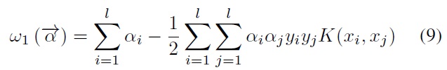
where
where
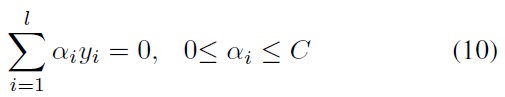
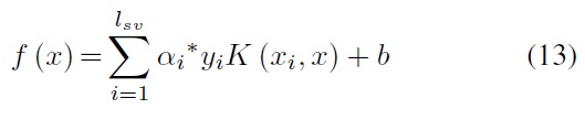
From Eq. (9), we can see that the size of the QP problem is equal to the number of training samples. SVMs are usually slow, especially for a large problem. Solving the above Lagrange multiplier, we can obtain the below decision function:
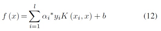
where
From Eq. (10), we know that 0 ≤
4. BCI Experiment for Motor Imagery EEG Classification
In this study, we used the BCI competition III-dataset IVa in which five subjects (aa, al, av, aw, and ay) imagined a right hand and foot movement. We also used the BCI competition IV dataset I, which involved four subjects (a, b, f, and g); two of them imagined a right and left hand movement, and two others imagined a left hand movement and foot movement. BCI III contained 280 trials for each subject, and BCI IV contained 200 trials for each subject. All the datasets were normalized to 59 electrodes, and the epoch time was selected from 0?4 seconds, for which the stimuli was given to subjects at 0 second. The raw signals were segmented from 1 second before the cue onset (0 second) and 4 second after the cue onset, so in total, they

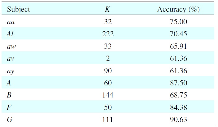
Experimental results of model selection for each subject with its best classification accuracy
included 5 second long time intervals from 59 channels. As the result, the power feature of the original signal
can be regarded to have a dimension of [59 × 2 × 7].
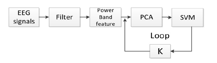
Figure 3 illustrates the generalized process for discriminant feature selection with
have a dimension of [59 × 2 × 7], so we have to find the dimensionality-reduced discriminant feature vector from them.

Table 1 shows the results of model selection of each subject with its best classification accuracy on the validation set. Because of individual differences, every subject has a different value of
For example, when subject aa has
This means the 32nd dimension contains 75% of the total features. We can see that the EEGs are subject-dependent, and the value of
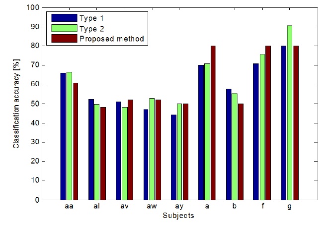
As shown in Figure 4, the proposed method outperformed the other methods. In case of type 1, it outperformed for subjects av, aw, ay, a, and f, and in the case of type 2, it outperformed for subjects al, ay, b, and g. The proposed method outperformed both the type 1 and type 2 methods.
To simplify the complexity of motor imagery EEG analysis in BCI systems, we proposed a discriminant feature selection method for motor imagery using an EEG-based BCI system. The proposed method is based on PCA and SVM. By applying PCA, we can successfully achieve our goal for discriminant feature selection, which is to decorrelate the original dataset of motor imagery EEGs and reduce its dimensionality while maintaining the discriminants. The selected features are in the form of a final feature vector set that we apply using a SVM as a classifier. By comparing the proposed method to previous methods, we found that the proposed method enhanced the availability of features up to 8% for each subject.
In the future, we will investigate other approaches for optimal feature selection without loss of performance. Although the proposed method improved the classification progress, the accuracy of the classification did not reach our goal. To improve the overall classification performance, we will study non-linear dynamical analysis approaches instead of stochastic analysis for brain signals.
No potential conflict of interest relevant to this article was reported.