1. Introduction and Related Work
The authors of [1] presented a method for determining the hand-eye calibration that employs an
The bearing-only measurements available from monocular cameras define a measurement function that is not invertible. That is, a 3-dimensional (3D) landmark in the world produces a 2-dimensional (2D) pixel-coordinate measurement. This function cannot be inverted such that the 2D pixel coordinates produce the 3D coordinates of a landmark. Therefore, according to [4], “a full Gaussian estimate of its state cannot be computed from the [measurement].” The very concept of a non-invertible function is not a sensible statement in a Bayesian framework such as the Kalman filter. The state vector defines a mean, and the covariance matrix defines a distribution about that mean to define a full probability density function. A method of determining the probability density function of a non-invertible bearing-only measurement of a 3D landmark is required. Strategies for solving the problem of including new landmarks in this scenario generally fall into two categories: delayed and undelayed.
Within the
Another delayed landmark initialization approach described in [6] is able to cope with features regardless of whether discernible parallax is observed over multiple observations. This implies that the method can deal with features that are effectively at an infinite distance. The authors of [6] solved the parametrization difficulties by reducing the initial uncertainty in landmark depth before including it in the filter. Their method required additional observations of the landmark with either a parallax that exceeds some threshold or a baseline distance that exceeds some threshold.
An early
The authors of [8] modified and extended the work of [7] by defining the initial observation ray as a conic probability density function.
A final example of an undelayed landmark initialization technique is that made possible through the inverse depth parametrization presented in [3]. This technique has the clear advantage of requiring far less space in the state vector and state covariance matrix, as it requires only six state elements per landmark, as compared to the potentially unlimited number of elements required for hypothetical-land mark-based methods. However, it has been noted in the literature that a negative inverse depth is a possible result of this parametrization, something that must be avoided. In this paper, we propose an approach that attempts to avoid completely the possibility of negative depth occurring.
The remainder of this paper is structured as follows. In Section 2., we briefly recall the UKF as proposed in the literature. In Section 3., we describe the novel landmark initialization technique, and in Section 4., related experiments. These lead to improved initializations; see Section 5.. In Section 6., we present our conclusions.
2. Monocular Camera Localization by UKF
The first sensor module is the IMU which is composed of an accelerometer array and a gyroscope array. The other sensor module is the camera, which we assume to be calibrated prior to any attempt to estimate the state of the total system. These two sensor modules define two coordinate systems, and the world coordinate system constitutes a third. The IMU coordinate system has its origin at the centre of the IMU body with each of its axes aligned with the relevant individual sensor. The camera’s coordinate system has the focal point as its origin with the
The state which is to be estimated must not only contain the properties of direct interest (i.e., the position and direction of the camera) but those elements which are necessary for the prediction of the system’s state at some time in the future, as well as the characterization of time varying IMU biases.
Measurements, inputs and predictions of state all occur at discrete time intervals. The prediction of state in a moving system therefore requires that some assumption be made which accounts for the unobserved motion between these observations. There are several models to choose from, including constant position, acceleration, and velocity models. These are so named for their assumption of what goes on during the unobserved time periods. The system either maintains its previous position (usually driven by some noise), maintains its last observed acceleration, or continues on at the previous best estimate of the system’s velocity. In the case of a platform which is intended to undergo motion associated with a vehicle or relatively smooth handheld motion, the constant velocity model is a common choice, and the one which is employed here.
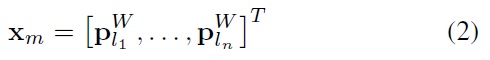
In a translating and rotating system whose motion is being estimated according to the constant velocity model, the motion values which predict the future state of the system are the translational and angular velocities. Angular velocity information is directly available from the gyroscope array, and so its inclusion in the system state is unnecessary. Translational velocity is not, however, directly measurable from the accelerometer array. The acceleration measurements it provides must be integrated over time to produce a translational velocity estimate. We may then define the portion of the system state which contains the relevant camera and IMU values as

where

is the vector containing the three Cartesian coordinates defining the position of the IMU in the world coordinate system. The direction of the IMU in the world frame is defined by the unit quaternion

The velocity of the entire strapdown system is defined by the vector v

defining the relative direction.
The final two elements b
The covariance matrix for the sensor state was found to be acceptably initialized to almost any small, positive, diagonal matrix. The state vector so far includes all values relevant to the camera and inertial sensors, however it does not yet contain any information about the state of the environment, most notably the static landmarks which will aid in the localization of the camera.
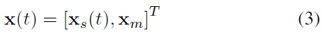
A single landmark can be defined in terms of the location from which it was first observed, a direction from that location towards the landmark, and its inverse depth. So the
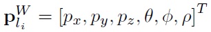
where the first three elements define the focal point of the camera when the landmark was first observed,
The entire state vector of the sensors and their environment can thus be described as
The Kalman filter framework is composed of a
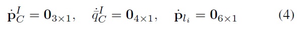
Elements of the state which change deterministically over time have derivatives
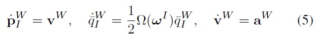
where the function Ω(
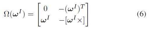
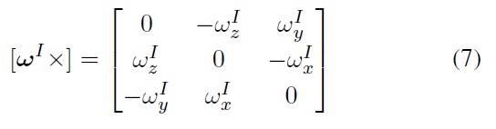
Here, [
The remaining accelerometer and gyroscope array biases, b
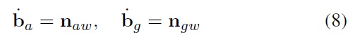
The measurements from the accelerometers and gyroscopes are also assumed to be corrupted by zero-mean Gaussian noise. These noise elements are termed n
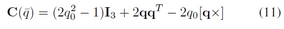
where

is the direction cosine matrix of the unit quaternion. A unit quaternion

“represents a rotation by the angle
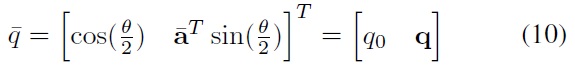
Given the above definition it is possible to define the matrix

as
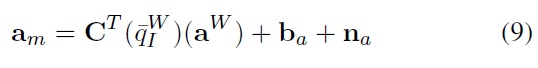
The angular velocity measurement is similarly defined as
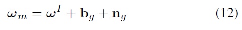
Algebraic rearrangement yields the values in the appropriate coordinate systems and with the noise and biases removed, as in

In this way the measurements from the accelerometers and gyroscopes can be included in the process update of the Kalman filter as control inputs.
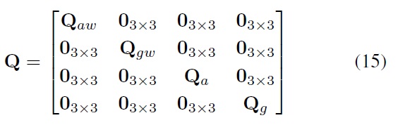
The process noise is therefore composed of two elements which drive the random walk of the internal sensor biases, and two elements which corrupt the measurements from the inertial sensors for a total of four vector elements which can be stacked into a process noise vector n where
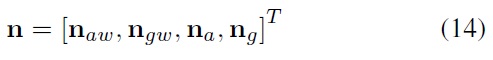
Each of the 3 × 1 noise vector elements has an attendant 3 × 3 covariance matrix termed, Q
Normally, it would be necessary to also attempt to estimate the direction of the gravity acceleration vector so as to remove its influence from the acceleration measurements. However, in Eq. (13) we see that the true state of accelerations does not have a vector representing gravity removed from it. This step is not necessary in this special case because the mobile phone in question already provides acceleration measurements with the influence of gravity removed.
The
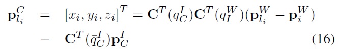
This prediction is based on the customary projection of a landmark onto the camera’s image plane. As the landmarks presented here are represented in the 6-dimensional inverse depth parametrization, it is first necessary to convert this representation into the customary 3-dimensional Cartesian representation. If we define a 3D Cartesian landmark in the world coordinate system as

then we can convert this representation to the camera’s coordinate system through
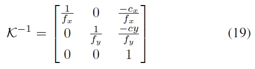
This landmark can then be projected onto the image plane www.ijfis. using the intrinsic camera matrix
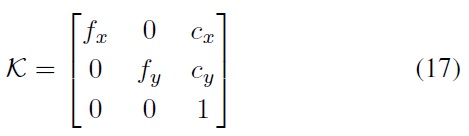
where
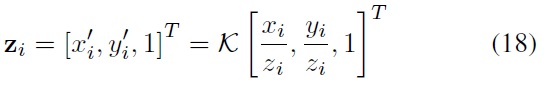
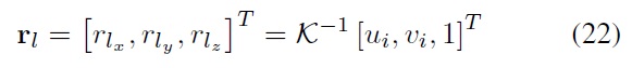
We can convert the pixel coordinates into a directional vector through use of the inverse of the intrinsic camera matrix where
The measurement then provided to the filter is z´
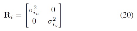
where
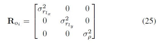
represent the variances in the horizontal and vertical components of the direction observation vector respectively. When multiple landmarks are observed, the covariance matrix for all landmark measurement noise is
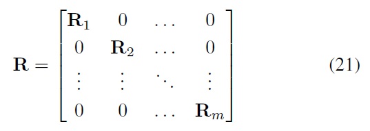
where
3. Novel Landmark Initialization
The addition of landmarks into the system state is problematic, as the covariance values which define the certainty of its initialization must be stated in terms of the certainty of all the other elements of the system. Each landmark is explicitly defined in terms of the position and direction of the camera at its first observation.
The covariance representing the certainty of the estimation of camera pose, must be related to the initial covariance of the landmark, particularly the origin and direction elements of the inverse depth parametrization. Likewise the certainty of the camera’s position and direction is related to the certainty of the estimation of the landmarks encountered so far. So, the initialization of the covariance of landmark must have important off-diagonal elements which relate it’s initial estimation to the current estimation of the device state and all previously initialized landmarks.
The EKF approach to initialization of landmarks [2] involves a first-order linearisation of the landmark-initialization function in order to fill the off-diagonal covariance elements related to the position and direction of the camera. The use of the Jacobian is a natural approach in the EKF framework as that is the general approach used for the process update as well. However, the UKF replaces this linearisation approach with the
For approaches using the UT for landmark initialization, see [10] (a delayed landmark initialization approach within the context of a SRUKF) and [11]. In [12] the authors claim to use an inverse depth parametrization of landmarks in the UKF framework but provide no indication of how they initialize their landmarks.
The general approach employed here is an adaptation of that used in [10], but with the added benefit that landmark initialization is undelayed. This is, after all, one of the key benefits of the parametrization according to [13]. The key observation of [10] is that the function, which takes the input of an observation in the form of pixel coordinates and transforms it to the inverse depth parametrization, is a non-linear function. Furthermore, when adding a landmark to the state, the desired information is the new state and state covariance after the application of this non-linear function. This is precisely the role of the UT. It takes a non-linear function, a state vector, and a covariance matrix and produces the new state and covariance, just what is wanted in the case of landmark initialization.
To be specific, we define the vector pointing in the direction of the new landmark as r
where [
Its initial inverse depth is unknown, so one is chosen arbitrarily. So the initial observation of a landmark
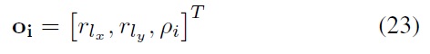
where
The state covariance matrix is likewise augmented. The covariance of the landmark observation is composed of the variance of the horizontal component of
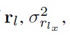
the variance of the vertical component of

and the variance of the inverse depth

resulting in the covariance matrix
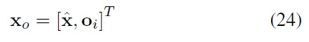
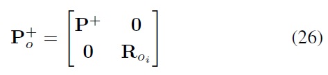
The state covariance matrix is then augmented with R
The non-linear function, which is used to add a landmark, can be defined as

where
With the state, covariance, and function defined, application of the UT is possible. Given a calibrated camera the variances of the horizontal and vertical landmark direction components defined in Eq. (25) will be small, on the order of fractional pixel dimensions. On the other hand, given that a landmark has only been observed a single time by a single camera, the inverse depth variance should be very large; theoretically it should be infinite.
This theoretically accurate characterization of depth can lead to at least two undesirable scenarios described below.
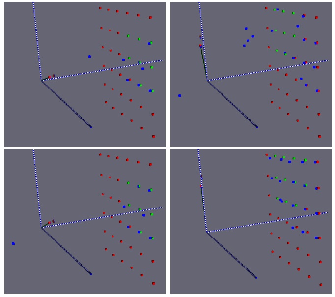
Because the initial depth is indicated to be totally untrustworthy, early measurements carry heavy weight. There are two possible problematic scenarios for the first two noisy observations of a landmark. In the first scenario illustrated in Figure 1, a noisy measurement may indicate that the landmark should in fact be much closer to the camera than its initial depth indicated.
From left to right in Figure 1, a single landmark (the upperleft green cube) is first observed and initialized at an arbitrary depth which is closer than its true depth (the blue cube which is farthest to the left). In the next image, it is then observed a second time, however, due to a noisy measurement its corrected position places it behind the camera. Then we see a cluster of landmarks which have been initialized together, and which due to some noise in either the camera position or in the pixel measurements themselves, were falsely given a high depth certainty after only two observations. Finally we see a case in which noise injection causes the previously problematic landmarks to correctly converge to their true positions.
The first scenario will result in a large correction from the Kalman gain matrix moving the landmark towards the camera. In some cases this correction is so large that the landmark moves to a position which is behind the camera, a behaviour also noted by [14]. Once the landmark is behind the camera, comparison of landmark measurements is no longer meaningful. The landmark’s continued presence in the filter negatively
influences the estimation of the position of other landmarks and thus the pose of the camera.
In the second problematic scenario, the second noisy measurement of the just initialized landmark erroneously confirms the initial depth. So the associated inverse depth variance suddenly changes from a very large value to a small value. Now the state covariance’s indication of landmark depth certainty will take precedence over the value indicated by observation.
The solution used here was to more closely control the characterization of the inverse depth of landmarks at the early stages of their inclusion in the state and state covariance of the filter. This combines the benefits of undelayed initialization, (i.e., the landmarks immediately contribute to and are included in the filter), with the benefits of delayed initialization, higher certainty that landmarks will converge smoothly to their true positions.
Instead of initializing landmarks with highly uncertain inverse depths, their depths are instead initialized with relatively high certainty. This approach, if left on its own, sometimes leads to the desired behaviour of dependable landmark convergence, however it also leads to a higher incidence of landmarks which tend to remain in their initial positions and only converge over a series of many observations as illustrated in Figure 1.
In order to alleviate this issue, landmarks are treated not as entirely stationary during a small, finite number of filter iterations after initialization. Instead, a small amount of noise is artificially injected into the inverse depth of new landmarks via the process covariance matrix. This approach results in a tunable landmark initialization process. The number of iterations that a landmark has noise injected into its inverse depth and the magnitude of this noise can be adjusted to produce different landmark convergence behaviours. In Figure 1, inverse depth noise has been injected for several filter steps resulting in properly initialized features with none behind the camera, and with none maintaining their initial wrong depth.
The initial covariance matrix values have a wide range of acceptable values (a feature which is not present in many other Kalman filter-based SLAM implementations). The identity matrix scaled by a small value (between 0 and 1) is sufficient. The landmark initialization technique accounts for the rest of the covariance matrix as landmarks are added. Covariance values for pixel noise are determined by offline camera calibration. The initial inverse depth covariance can also occupy the same very wide range mentioned for noise injection in Eq. (29).
Depending on the desired convergence behaviour, a high number of initialization iterations may be used with a small noise value, or a small number of iterations may be combined with a relatively large amount of noise. In the first case, convergence happens in a slower but more controlled manner which ultimately tends to arrive at a more accurate initialization of the landmark. However, this approach relies on a scenario in which new features are assumed to be visible for a large number of iterations.
If a reliance on many observations of a landmark during initialization is assumed, and this requirement is not met, it is likely that no landmarks will converge quickly enough to their true positions and so no true landmark positions will be known. This will often lead to filter divergence, or in the best case a filter which diverges, but has drifted by some significant translation and rotation from the true world pose.
In the second case, large noise injections for a small number of iterations tend to produce a lower quality initial estimate for the landmark, but it converges to the general neighbourhood of the true position more quickly and so is suitable for landmarks which may only be observed for a short period of time. As the magnitude of noise injected increases, the likelihood of a landmark being estimated to be behind the camera increases, so a balance must be maintained between speed and reliability of convergence.
The noise, which is added to the inverse depth values of landmarks during their initialization period, is accomplished as part of the process update step through modification of the process covariance Q from Eq. (15). If the number of landmarks which have not completed their required number of initialization steps is
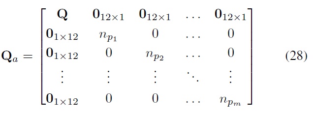
In Eq. (4) the derivatives of the landmarks in the state vector were defined as 0. However in the case of the
5. Improved Landmark Initialization
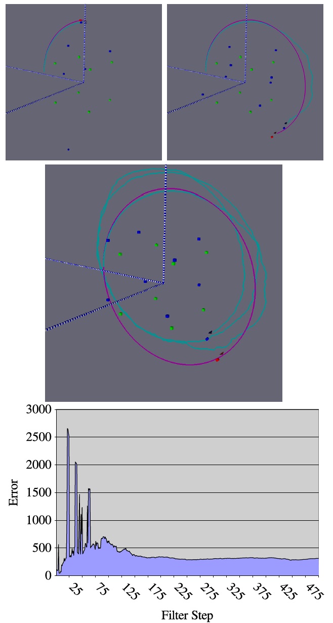
A major weakness of the landmark initialization approach described above is that both the number of steps for which noise is injected and the magnitude of that noise must be tuned to the scene in which the filter is operating. The characterization of the noise injection is largely dependent upon how many new landmarks are likely to be encountered at any given step, and how frequently these new bundles of landmarks will be encountered. In a simulated test scenario, aimed at determining the noise tolerance of the UKF, a simulated device continuously observed eight landmarks while rotating around them (identical to that pictured in Figure 2).
The maximum noise tolerance for the IMU elements was determined to be noise with a variance of 0.5 m/s-2 for the accelerometers and 50 radians/s for the gyroscopes. However, the particular noise injection settings that were effective in this scenario were not at all effective for a noisy camera scenario. In fact, after extensive systematic testing using a variety of noise injection values, no combination of noise injection values was found to be capable of improving bearing measurement noise tolerance beyond a noise variance barrier of 0:4°, even in the case of a very-low-noise IMU.
Extensive observation of the behavior of landmarks early in their introduction to the system state has led to what may be a helpful description through an analogy of their behavior. Landmarks that have just been added to the filter behave as if they have mass and therefore inertia. They resist, to some degree, movement from their initial positions to their true positions. The force that acts on these masses to drive them toward their true locations is the noise that is injected. The mass of each landmark appears to be determined by two factors: the number of landmarks that are simultaneously being initialized, and the number of landmarks that have already been initialized. Of the two factors that contribute to a landmark’s resistance to motion, by far, the most important is the number of landmarks that are simultaneously initialized.
There exist two possible approaches to dealing with this behavior. One is to characterize a dynamic noise injection scheme that changes the magnitude and number of iterations for the noise, dependent upon the number of new landmarks and the number of already encountered landmarks. However, it appears that not all scenarios have a noise injection scheme that will yield acceptable results. The second approach is to define noise injection values for a particular scenario, and force the filter to encounter this scenario always. This second option has been implemented.
Regardless of how many new landmarks are encountered by the camera, the filter only allows one new landmark to be initialized every five filter steps. In this way, we fix the most
important factor determining landmark initialization behavior to a single scenario, that of initializing a single landmark. In the mass analogy above, this ensures very “light” landmarks that require little “force” to be moved toward their true position. After extensive testing in a wide range of scene configurations, it was found that the range of acceptable noise magnitudes was large. Any magnitude from
displayed acceptable and nearly identical behavior.
An undesirable consequence of forcing only a single landmark to be initialized at a time was the higher incidence of negative depth landmarks. By removing these landmarks from the UKF when encountered, convergence to the true state was attainable in all the encountered scene configurations with reasonable noise configurations. The removal of a landmark is trivial. It is removed from the state vector, and all rows and columns that are shared by the landmark in the state covariance matrix are removed.
By employing this method, the maximum allowable measurement noise variance for the test scenario described above was improved from 0:007 to 0:3 radians, or from 0:4° to 16:7°. We observed, as illustrated in Figure 2, that by approximately step 45 (or 10 steps after the final landmark was initialized), all 8 landmarks had been successfully introduced to the filter.
From left to right, we first see the state of the UKF at step 45. This is the step at which all landmarks have been added to the filter; however, we observe only five landmarks from the filter in the general neighborhood of the true landmarks. By step 125 in the next image, we see all landmarks in the filter have moved to the region around the true landmarks. By step 500, we see that filter landmarks have now converged to the correct shape, but both the path of the camera and the location of the landmarks according to the UKF have been shifted in the positive
The filter converges to a higher overall error value than that produced by the noisy IMU scenario; however, this error rate is somewhat misleading. Due to the high level of uncertainty in landmark positions in the early stages, the estimated state of the system is also uncertain in the early stages. This leads to an offset in both camera and landmark positions. That is, the whole-world coordinate system, including both the camera and landmarks, is translated by a constant amount relative to the true coordinate as illustrated in Figure 2. Depending on the application, error of this type may or may not be important. For example, indoor navigation and 3D scene reconstruction applications would not necessarily be adversely affected by a shift in the world coordinate system.
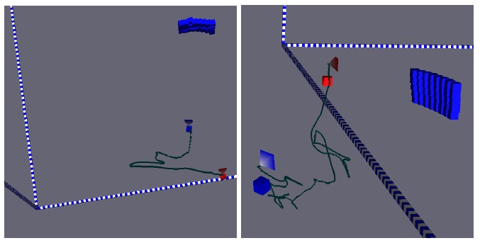
In two real-world experiments, approximately 1 min of video and IMU data were recorded. These took more than 8 h to process, and therefore, we have not yet recorded longer sequences.
However, in both cases, pictured in Figure 3, the locations of landmarks were accurately estimated with what appeared to be accuracy in the order of 1 mm.
The red cube and pyramid indicate the starting positions of the IMU and camera, respectively. The blue IMU and camera indicate the final position of the device. The real-world landmarks were the corners of an 8 × 5 planar calibration grid. The dimensions of each square were 4 cm × 4 cm. Each side of the blue landmark cubes also measured 4 cm. The close stacking of the cubes indicates accurate landmark position estimation. The landmark cubes are visualized as axis-aligned; this is not necessarily true in reality, as alignment of the image plane parallel to the calibration grid was not attempted. Some landmark cube overlap may therefore be attributed to improper cube alignment.
The motion of the device was not estimated very accurately; however, toward the end of the experiments, the device appeared to follow the actual motion of the experimental device closely, and the final position of the device appeared to approximate closely to that of the true system.
The early incorrect motion estimation results for the 1-min sequences are probably the result of the poor noise and bias estimation frequently observed during early state convergence. These low-quality results were also seen in the early stages of the simulations, as seen in Figure 2. The simulations were much faster to process, and therefore we could afford to perform many more iterations. The convergence of landmarks and proper motion of the device toward the end of the real-world experiments tends to indicate that the UKF is performing properly. Longer recorded sequences with some estimation of the real-world ground truth are needed to verify this claim.
Furthermore, we have so far relied on the observation of calibration grids for the reliable repeated observation of landmarks. In order to generalize this approach to markerless scenarios, a reliable landmark observation technique is needed.
No potential conflict of interest relevant to this article was reported.