This paper presents a stochastic driver behavior modeling framework which takes into account both individual and general driving characteristics as one aggregate model. Patterns of individual driving styles are modeled using a Dirichlet process mixture model, as a non-parametric Bayesian approach which automatically selects the optimal number of model components to fit sparse observations of each particular driver’s behavior. In addition, general or background driving patterns are also captured with a Gaussian mixture model using a reasonably large amount of development data from several drivers. By combining both probability distributions, the aggregate driver-dependent model can better emphasize driving characteristics of each particular driver, while also backing off to exploit general driving behavior in cases of unseen/unmatched parameter spaces from individual training observations. The proposed driver behavior model was employed to anticipate pedal operation behavior during car-following maneuvers involving several drivers on the road. The experimental results showed advantages of the combined model over the model adaptation approach.
Predicting driving behavior by employing mathematical driver models, which are obtained directly from the observed driving-behavior data, has gained much attention in recent research. Various approaches have been proposed for modeling driving behavior based on different interpretations and assumptions, such as the piecewise autoregressive exogenous (PWARX) model [1,2], hidden Markov model (HMM) [3], neural network (NN) [4], and Gaussian mixture model (GMM) [5]. These approaches have reported impressive performance on simulated and controlled driving data. Some of these promising techniques exploit a set of localized relationships to model driving behavior (e.g., mixture models, piecewise linear models). These models assume that the observed data are generated by a set of latent components, each having different characteristics and corresponding parameters. Therefore, complex driving behavior can be broken down into a reasonable number of sub-patterns. For instance, during car following, it is believed that drivers adopt different driving patterns or driving modes (e.g., normal following, approaching) under different driving situations, depending on individual and contextual factors. One challenge in behavior modeling is to determine how many latent classes or localized relationships exist between the stimuli and the driver’s responses (i.e., model selection problem), and to estimate the properties of these hidden components from the given observations. In general, a trade-off in selecting the number of components arises: with too many components, the obtained model may over-fit the data, while a model with too few components may not be flexible enough to represent an underlying distribution of observations.
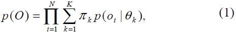
A finite GMM [6] is a well-known probabilistic and unsupervised modeling technique for multivariate data with an arbitrarily complex probability density function (pdf). Expectation-maximization (EM) is a powerful algorithm for estimating parameters of finite mixture models that maximizes the likelihood of observed data. However, the EM algorithm is sensitive to initialization (i.e., it may converge to a local maximum), and may converge to the boundary of a parameter space, leading to a meaningless estimate [6]. Moreover, EM provides no explicit solution to the model selection problem, and may not yield a wellbehaved distribution when the amount of training data is insufficient.
Recently, the Dirichlet process mixture model (DPM), a non-parametric Bayesian approach, has been proposed to circumvent such issues [7,8]. Unlike finite mixture models, DPM estimates the joint distribution of stimuli and responses using a Dirichlet process mixture by assuming that the number of components is random and unknown. Specifically, a hidden parameter is first drawn from a base distribution; consequently, observations are generated from a parametric distribution conditioned on the drawn parameter. Therefore, DPM avoids the problem of model selection by assuming that there are an infinite number of latent components, but that only a finite number of observations could be observed. Most importantly, DPM is capable of choosing an appropriate number of latent components to explain the given data in a probabilistic manner. DPM has been successfully applied in several applications such as modeling content of documents and spike sorting [7,9].
In car following, driver behavior is influenced by both individual and situational factors [10,11]; hence, the best driver behavior model for each particular driver should be obtained by using individual observations that include all possible driving situations. However, at present, it is not practical to collect such a large amount of driving data from one particular driver in order to create a driver-specific model. To circumvent this issue, a general or universal driver model, which is obtained by using a reasonable amount of observations from several drivers, is used to represent driving behavior in a broad sense (e.g., average or common relationships between stimuli and responses). Subsequently, a driver-dependent model can be obtained using a model adaptation framework that can automatically adjust the parameters of the universal driver model by shifting the localized distributions towards the available individual observations [5].
In this paper, we proposed a new stochastic driver behavior model that better represents underlying individual driving characteristics, while retaining general driving patterns. To cope with sparse amounts of individual driving data and the model selection problem, we employed DPM to train an individual driver behavior model in order to capture unique driving styles from available observations. Furthermore, in order to cope with unseen or unmatched driving situations that may not be present in individual training observations, we employed a GMM with a classical EM algorithm to train a universal driver model from observations of several drivers. Finally, the driver-dependent model is obtained by combining both driver models into one aggregate model in a probabilistic manner. As a result, the combined model contains both individual and background distributions that can better represent both observed and unobserved driving behavior of individual drivers.
Experimental validation was conducted by observing the car-following behavior of several drivers on the road. The objective of a driver behavior model is to anticipate carfollowing behavior in terms of pedal control operations (i.e., gas and brake pedal pressures) in response to the observable driving signals, such as the vehicle velocity and the following distance behind the leading vehicle. We demonstrated that the proposed combined driver model showed better prediction performance than both individual and general models, as well as the driver-adapted model based on the maximum a posteriori (MAP) criterion [5].
II. CAR FOLLOWING AND DRIVER BEHAVIOR MODEL
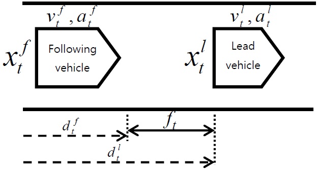
Car-following characterizes longitudinal behavior of a driver while following behind another vehicle. In this study, we focus on car following in the sense of the way the behavior of the driver of a following vehicle is affected by the driving environment (i.e., the behavior of the leading vehicle) and by the status of the driver’s own vehicle. There are several contributory factors in car-following behavior such as the relative position and velocity of the following vehicle with respect to the lead vehicle, the acceleration and deceleration of both vehicles, and the perception and reaction time of the following driver.
Fig. 1 shows a basic diagram of car following and its corresponding parameters, where
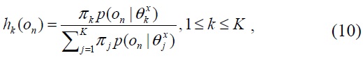
In general, a driver behavior model predicts a pattern of pedal depression by a driver in response to the present velocity of the driver’s vehicle and the relative distance between the vehicles. Subsequently, the vehicle velocity and the relative distance are altered corresponding to the vehicle dynamics, which responds to the driver’s control behavior of the gas and brake pedals. Most conventional carfollowing models [12-14] ignore the stochastic nature and multiple states of driving behavior characteristics. Some models assume that a driver’s responses depend on only one stimulus such as the distance between vehicles. In this study, we aim to model driver behavior by taking into account stochastic characteristics with multiple states involving multi-dimensional stimuli. Therefore, we adopt stochastic mixture models to represent driving behavior.
III. STOCHASTIC DRIVER MODELING
The underlying assumption of a stochastic driver behavior modeling framework is that as a driver operates the gas and brake pedals in response to the stimuli of the vehicle velocity and following distance, the patterns can be modeled accordingly using the joint distribution of all the correlated parameters. In the following subsections, we will describe driver behavior models based on GMM, DPM, and the model combination.
In a finite mixture model, we assume that
The observed data are generated from a mixture of these multiple components. In particular, the total amount of data generated by component
where
In general, the hidden parameters (
>
B. Dirichlet Process Mixture Model
By adopting a fully Bayesian approach, DPM does not require
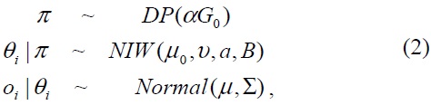
where
where NIW is represented by a mean vector
where
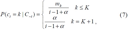
indicates the component ownership or mixture index of each observation. One can obtain samples from this distribution using Markov chain Monte Carlo (MCMC) methods [8], particularly Gibbs sampling, in which new values of each model parameter are repeatedly sampled, conditioned on the current values of all the other parameters. Eventually, Gibbs samples approximate the posterior distribution upon convergence. As a result, this avoids the problem of model selection and local maxima by assuming that there are an infinite number of hidden components, but only a finite number of which could be observed from the data.
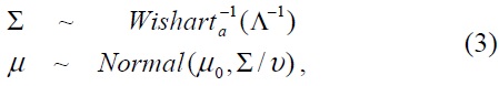
As the state of the distribution consists of parameters
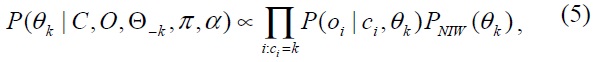
where Θ

where
where
>
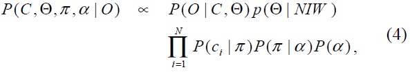
C. Maximum A Posterior Adaptation
Also known as Bayesian adaptation, MAP adaptation reestimates the model parameters individually by shifting the original statistic toward the new adaptation data. Given a set of adapting data, {
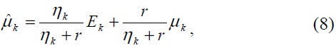
where,
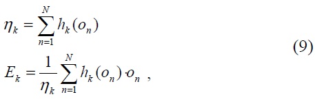
where
where
is the marginal probability of the observed parameter
The adapted model is thus updated so that the mixture components with high counts of data from a particular characteristic/correlation rely more on the new sufficient statistic of the final parameters. More discussion of MAP adaptation for a GMM can be found in [16].
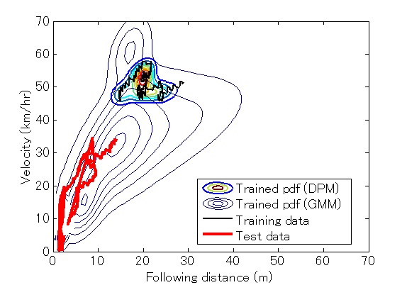
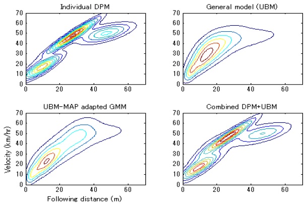
Fig. 2 illustrates an example of an observed driving trajectory (solid line) overlaid with a corresponding pdf generated by the well-trained DPM (the smaller pdf plot). The bigger pdf plot in the background represents a general joint distribution (e.g., the universal driver model). The dotted line represents an unseen car-following trajectory during the validation stage. As we can see, the individual driver model obtained using a DPM is better at modeling the joint probability of the observed driving trajectory than the universal background driver model. However, the individual model is focused on parameter space that does not cover the test driving trajectory, and hence cannot represent unseen driving behavior. Although not particularly optimized for this particular driver, the universal background model can better represent common driving behavior in most situations.
By combining these two probability distributions into a single aggregate distribution, the resulting driver-dependent model can better represent individual driving characteristics that were previously observed by the individual distribution (Θindividual), as well as explain unseen driving characteristics by the background distribution (Θgeneral). In this study, we apply weighted linear aggregation of two probability distributions as

where 0 ≤
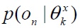
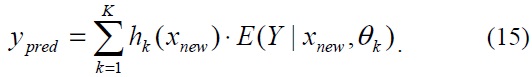
In a regression problem, an observation consists of both input stimuli and output responses (
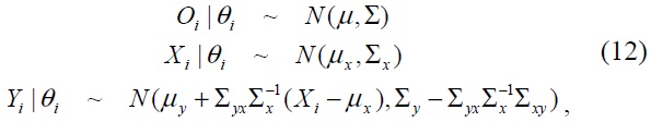
where the mean vector
Thus, the optimal prediction of the observation

Consequently, the predicted responses
The driving signals utilized are limited to following distance (m), vehicle velocity (km/hr), and gas and brake pedal forces (N), obtained from a real-world driving corpus [18]. All the acquired analog driving signals from the sensory systems of the instrumented vehicle are re-sampled to 10 Hz, as well as rescaled into their original units. The offset values caused by gas and brake pedal sensors are removed from each file, based on estimates obtained using a histogram-based technique. Furthermore, manual annotation of driving-signal data and driving scenes was used to verify that only concrete car-following events with legitimate driving signals that last more than 10 seconds are considered in this study. Cases where the lead vehicle changes its lane position, or another vehicle cuts in and then acts as a new lead vehicle are regarded as two separate car-following events. Consequently, the evaluation is performed using approximately 300 minutes of clean and realistic carfollowing data from 64 drivers. The data was randomly partitioned into two subsets of drivers for the open-test evaluation (i.e., training and validation of the driver behavior model). All the following evaluation results are reported as the average of both subsets, except when stated otherwise.
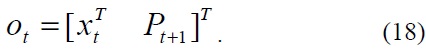
In this study, an observed feature vector (stimuli) at time

where the Δ(·) operator of a parameter is defined as
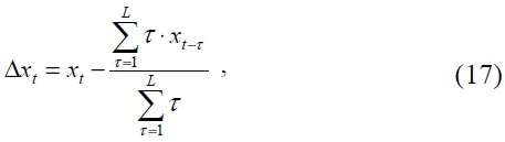
where
>
C. Signal-to-Deviation Ratio
In order to assess the ability of the driver behavior model to anticipate pedal control behavior, the difference between the predicted and actually observed gas-pedal operation signals is used as our measurement. The signal-to-deviation ratio (SDR) is defined as follows
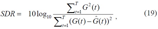
where
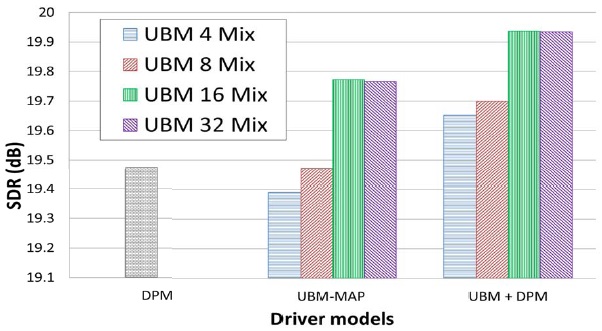
First, the individual driver model is obtained by training a DPM with individual driving data [19]. Again, a DDPM automatically selects the appropriate number of mixture components that best fits the training observations. Next, the general driver models or universal background models (UBM) were obtained by employing the EM algorithm, using driving data from a pool of several drivers in the development set. In this study, we prepared the UBMs with 4, 8, 16, and 32 mixtures for comparison. Subsequently, a driver-dependent model is obtained by merging the DPM-based individual driver model and the general driver models (UBMs).
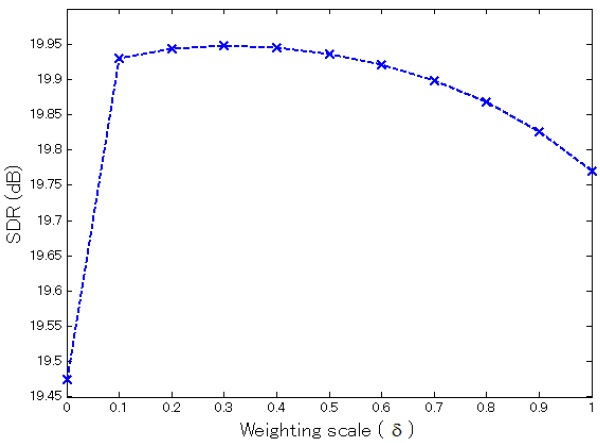
Fig. 3 shows the prediction performance of the proposed combined models using a 16-mixture UBM with different weighting scales (i.e.,
Fig. 4 illustrates example pdfs generated by an individual model (DPM), general model (UBM), driver-adapted model (UBM-MAP), and combined model (UBM+DPM). Finally, Fig. 5 compares the gas-pedal prediction performance off various driver models based on a DPM , UBM-MAP adaptation (with 4, 8, 16, and 32 mixtures), and the proposed combined DPM-UBM models obtained from the same UBM sets.
In contrast to the EM-based individual driver model, the driver-adapted (UBM-MAP) models tended to have better performance as the number of mixture components increased. This is because a reasonable amount of training data is needed to train a well-defined UBM, and some local mixtures were then adapted to better fit individual driving characteristics. When we combined the UBMs with the DPM-based individual model, the prediction performance was better than the driver-adapted (UBMMAP) model. The best performance was obtained by combining the 16-mixture UBM with DPMs that contained approximately 10 mixtures per driver on the average. Although the total number of components in the combined model is more than the original UBM, the achieved performance is considerably better than the 32-mixture UBM-MAP adapted model with fewer total mixtures (26 mixtures per driver on average).
In this paper, we presented a stochastic driver behavior model that takes into account both individual and general driving characteristics. In order to capture individual driving characteristics, we employed a DPM, which is capable of selecting the appropriate number of components to capture underlying distributions from a sparse or relatively small number of observations. Using different approach, a general driver model was obtained by using a parametric GMM trained with a reasonable amount of data from several drivers, and then employed as a background distribution. By combining these two distributions, the resulting driver model can effectively emphasize a driver’s observed personalized driving styles, as well as support many common driving patterns for unseen situations that may be encountered. The experimental results using on-the-road car-following behavior showed the advantages of the combined model over the adapted model. Our future work will consider a driver behavior model with tighter coupling between individual and general characteristics, while reducing the number of model components used, in order to achieve more efficient computation.