This paper proposes an efficient hardware architecture for high efficiency video coding (HEVC), which is the next generation video compression standard. It adopts several new coding techniques to reduce the bit rate by about 50% compared with the previous one. Unlike the previous H.264/AVC 6-tap interpolation filter, in HEVC, a one-dimensional seven-tap and eight-tap filter is adopted for luma interpolation, but it also increases the complexity and gate area in hardware implementation. In this paper, we propose a parallel architecture to boost the interpolation performance, achieving a luma 4×4 block interpolation in 2?4 cycles. The proposed architecture contains shared operations reducing the gate count increased due to the parallel architecture. This makes the area efficiency better than the previous design, in the best case, with the performance improved by about 75.15%. It is synthesized with the MagnaChip 0.18 μm library and can reach the maximum frequency of 200 MHz.
High efficiency video coding (HEVC) [1], which will be finalized in 2013, is the most recent joint video project of the Joint Collaborative Team on Video Coding (JCT-VC). The purpose of HEVC is to save the bit-rate by about 50% compared with the previous H.264/AVC standard [2], and it is targeted for up to ultra high-definition (UHD, 7680×4320) resolution. For the previous H.264/AVC standard, a number of studies have been performed, such as [3-5]. However, the research for HEVC remains insufficient, especially regarding hardware design.
HEVC allows for various new coding techniques, such as 35 luma intra-prediction modes, spatial and temporal MV prediction for inter-prediction, 4×4 discrete sine transform (DST), and sample adaptive offset (SAO) for a deblocking filter.
In this paper, we propose a hardware interpolation architecture for inter-prediction. In H.264/AVC, six-tap and linear filters are used for luma interpolation. However, unlike H.264/AVC, the interpolation in HEVC adopts onedimensional eight-tap and seven-tap interpolation [6]. Therefore, in the worst case, 11×11 reference pixels are used for a 4×4 luma interpolation. This increases the design complexity and the gate area when it is implemented into the hardware architecture.
In order to achieve high performance, we adopt a highly parallel architecture, which can increase the area. However, we also propose a shared operation processing element (PE) to reduce the area.
The rest of the paper is organized as follows. In Section II, the basic interpolation algorithm is briefly introduced. In Section III, the proposed architecture is presented. Section IV provides the final analysis and the conclusion is addressed in Section V.
Like H.264/AVC, the accuracy of motion compensation in HECV is 1/4 pel for luma samples. To obtain the noninteger luma samples, eight-tap and seven-tap interpolation filters are applied horizontally and vertically to generate luma half-pel and quarter-pel samples, respectively [7].
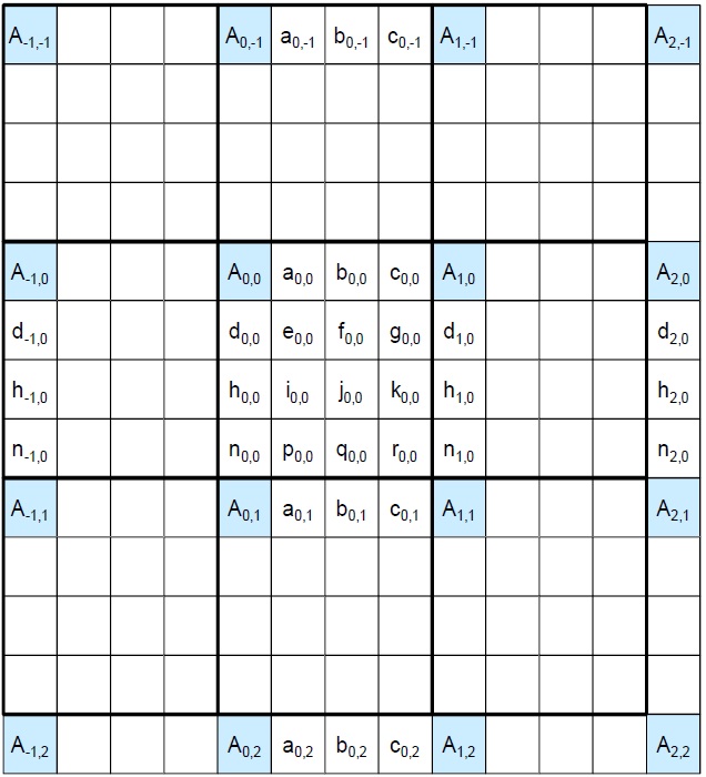
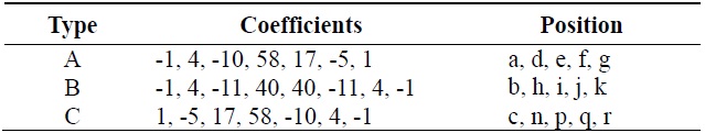
The fractional positions for HEVC inter-prediction luma interpolation are shown in Fig. 1, which is from HEVC draft 6 [1]. Capital letters in Fig. 1 indicate the integer samples used as reference pixels. Table 1 shows the coefficients used in the luma interpolation filters.
As shown in Table 1, the coefficients can be divided into three types. The a, d, e, f, and g positions use A type coefficients, while the b, h, i, j, and k positions use B type coefficients, and the c, n, p, q, and r positions use C type coefficients. The a, b, and c positions are filtered by applying horizontal filters and the d, h, and n positions are filtered by applying vertical filters. For calculating the other pixel values, both horizontal and vertical filters are used. For example, if the position we have to calculate is f, j, or q, vertical filters are used with the b position as the reference pixel. However, the b position should be calculated by applying horizontal filters in advance.
[Table 1.] Luma interpolation coefficients
Luma interpolation coefficients
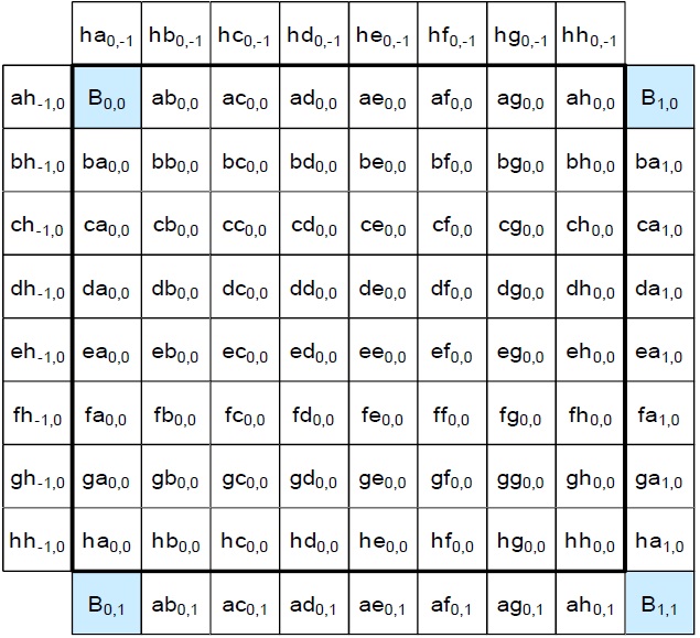
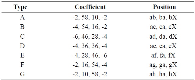
Fig. 2 shows the chroma fractional positions for HEVC inter-prediction interpolation. For the positions aX (X represents the letters from b to h) and Xa shown in Fig. 2 from HEVC draft 6 [1], horizontal filters and vertical filters are used for interpolation, respectively. For the other fractional positions, both horizontal filters and vertical filters must be used, as is done in the luma pixel filtering process. For example, the Xb positions should be calculated by applying vertical filters with the ab position as the reference pixel and the ab position should be calculated by applying a horizontal filter beforehand. Table 2 shows the coefficients used in the chroma interpolation filters.
[Table 2.] Chroma interpolation coefficients
Chroma interpolation coefficients
From Table 2 we can find out there are seven types of coefficients in chroma interpolation and the positions use the corresponding types of coefficients are also shown in Table 2. For example, the ab, ba, and bX positions use the A type filter with the coefficient of {-2, 58, 10, -2}.
In this section, we present the proposed interpolation architecture used for interpolation of HEVC inter-prediction.
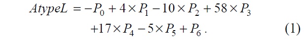
There are three types of coefficients in Table 1. However, we determined that if the order of the coefficients in the A type is reversed, the C type coefficients can be obtained. Therefore, if the order of input reference pixels is changed, the same hardware architecture can be used for both the A type and C type. In this way, we designed the A type and B type filters to form basic luma PEs. In the same way, we designed the A type, B type, C type, and D type to contain basic chroma PEs. Eqs. (1) and (2) show the original A type and B type luma filters.
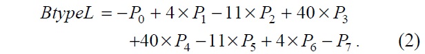
To eliminate the multiply operation in Eqs. (1) and (2), we converted them into Eqs. (3) and (4).
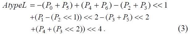
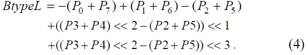
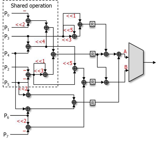
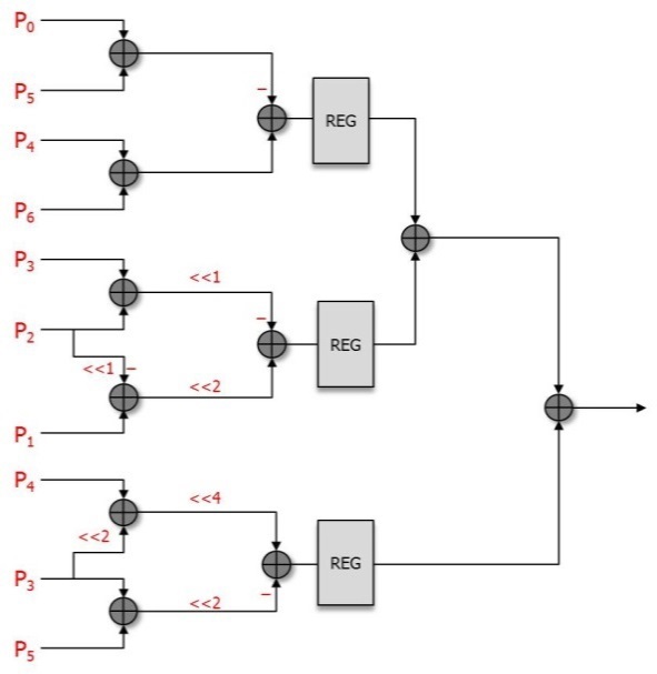
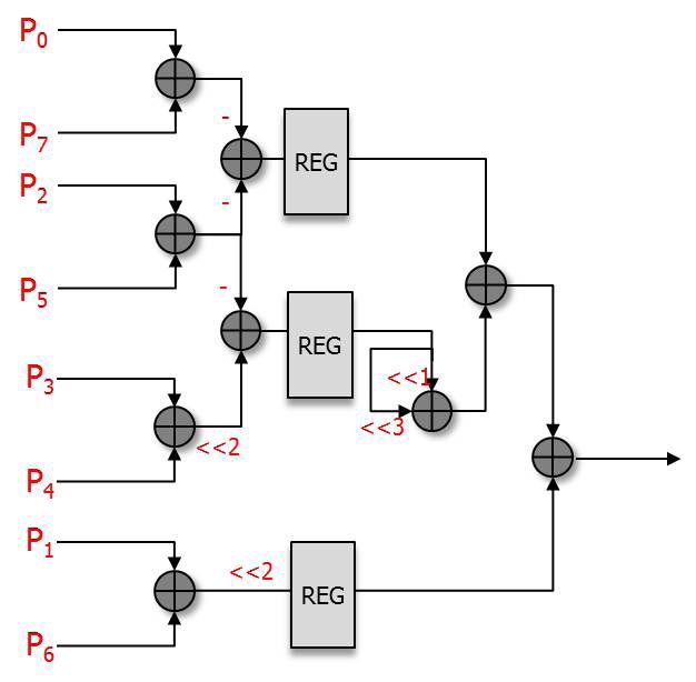
The luma A type PE and B type PE designed from Eqs. (3) and (4) are shown in Figs. 3 and 4.
Figs. 3 and 4 show that both the A type PE and B type PE consist of shift and additional operations. There are 11 and 9 adders in the A type PE and B type PE, respectively. To reduce the critical path, we have inserted registers so that we can boost the maximum frequency.
The hardware architecture that we propose introduces highly parallel architecture, which increases the gate count. In order to reduce the gate count, the separated A type PE and B type PE are combined into one shared operation filter that comprise a PE. The reason that they can be combined is that they are not used at the same time in the process of filtering.
We determined the common part from Eqs. (3) and (4) for shared operations.
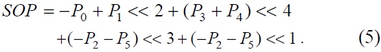
The shared operation (SOP) in Eq. (5) shows the common part used in both the A type filter and B type filter.
This SOP is used in Eqs. (6) and (7).
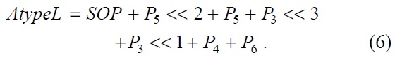
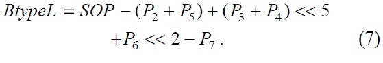
The original separated A type PE and B type PE have 20 adders in total. However, the combined filter with shared operation has 17 adders, which is 15% less than the previous ones in terms of additional operators.
For the chroma filter, a similar algorithm was applied. The equations for the chroma filter are shown below.
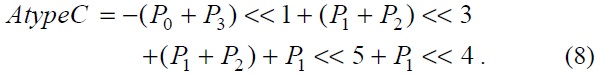
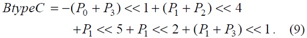
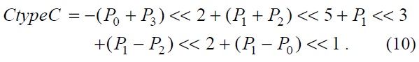
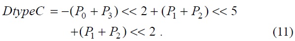
The equations, from Eqs. (8) to (11), show the chroma filters applied in the proposed architecture. In the chroma filter equations, the P0+P3 part and P1+P2 part can be used as shared operations.
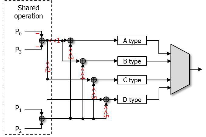
Table 3 shows the comparison of the operators used in several designs. The number of the operators shown in Table 3 is the sum of the operators in each luma PE and chroma PE. Draft [1] contains a large number of multiplier operators, and this greatly increases the gate count. However, the original design and the proposed design consist of adders and shifters to reduce the gate count. Figs. 5 and 6 show the proposed interpolation luma PE and chroma PE applied to the equations from Eqs. (6) to (11).
[Table 3.] Comparison of the number of operators
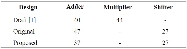
Comparison of the number of operators
Compared with the original PEs, the architecture shown in Figs. 5 and 6 can reduce the gate count by about 10%.
The proposed PEs shown in Figs. 5 and 6 can only predict one pixel value at a time. However, this does not meet the purpose of decoding 2560×1600 sized videos, which we used for the real-time test. Therefore, we decided to design a highly parallel architecture.
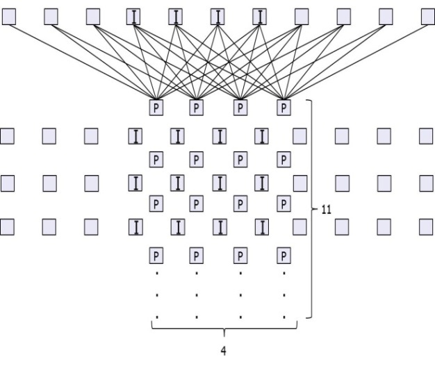
Fig. 7 shows the proposed parallel luma filter. The I positions in Fig. 7 show the integer positions in a 4×4 luma block. The P positions indicate the PEs in the proposed filter. There are 11 reference pixels since there are 8 reference pixels needed for each predicted pixel in the worst case, and there are 4 predicted positions in both directions. That means, for a luma 4×4 block, 11×11 reference pixels are needed. There are 4×11 PEs in total, and the luma filter can predict the a, b, c, d, h, and n positions in 2 cycles. In this case, the PEs from the 4th to 7th rows are used. In the other positions, all of the 4×11 PEs are used in the first two cycles and the PEs from the 4th to 7th rows are reused in the next two cycles.
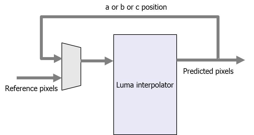
Fig. 8 shows the luma filter reuse block diagram. In the first two cycles, position a, b, or c is predicted, and the predicted pixels feed back to the input of the luma interpolator, as shown in Fig. 8. The chroma filter was designed by a similar method. For a chroma 2×2 block, 5×5 reference pixels are needed. There are 2×5 chroma PEs used as both horizontal and vertical filtersma filter needs 1?2 cycles to predict a chroma 2×2 block.
The proposed architecture was synthesized with the MagnaChip 0.18 μm library and can reach a frequency of 200 MHz. It has to achieve the processing of 2560× 1600×30+2560×1600×30×0.5 = 184320000 pixels in one second. In the worst case, for a luma 4×4 block and two chroma 2×2 blocks with bi-directional prediction, 4×2 = 8 cycles and 2×2+2×2 = 8 cycles are needed, respectively. Thus, 16 cycles in total are required to predict 16+8 = 24 pixels. Since it can process 24/16 = 1.5 pixels/cycle on average, and the minimum frequency needed is about 184320000/1.5 = 122 MHz, the proposed design, which has a higher frequency, can decode a 2560×1600 sized video in real-time.
For the luma interpolator, in the best case, it takes 2×2×16 = 64 cycles for one 16×16 block and the process of the pixel for each cycle is 256/64 = 4 pixel/cycle. The gate area of the proposed design is 84400, so the area efficiency is 4/84400 = 0.047 (pixel/cycle)/kgate.
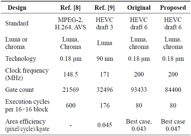
Table 4 shows the comparison of the synthesis result with previous designs. Zheng et al. [8] was designed with three different standards, so it is not accurate to compare the gate count. However, in terms of the number of cycles, the proposed design improved the performance by about 86.67%.
The design of Guo et al. [9] was based on HEVC draft 3, which has different coefficients from the working draft 6 we have applied, and it only implemented a luma interpolator. The proposed design has improved the performance by about 63.64% in terms of the cycle number compared with the design of Guo et al. [9]. Even though the gate area has been greatly increased, the area efficiency is better than that of Guo et al. [9] in the best case.
[Table 4.] Comparison of the synthesis results

Comparison of the synthesis results
In this paper, we proposed a highly parallel interpolation hardware architecture for both luma pixels and chroma pixels. It was designed with Verilog HDL and tested with the test vectors extracted from HM7.0. It was synthesized with the design compiler supported by the IC Design Education Center (IDEC). The synthesis results show the maximum frequency of the proposed design can reach up to 200 MHz. The experimental results showed that the proposed design improved the performance by about 75.15%, with an area efficiency better than previous designs in the best case.