In accordance with the increase of vehicles recently, traffic congestion has become a serious problem. In urban areas, almost all traffic congestion occurs at intersections. Intersections can be classified into three types according to the number of roads meeting at the intersection: T-junction (3-way intersection), Crossroads (4-way intersection), and Multi-way intersection (more than 4 ways). The traffic signal phases are generally more complicated at multi-way intersections and consequently traffic jams occur more easily. One of the ways to solve this problem is road expansion, but high costs and long construction periods make this option difficult in urban areas. In such cases, traffic signal control is a reasonable alternative method for reducing traffic jams.
Traffic signal controls can be classified into two types. One is an offline (pretimed) control and the other is an online (adaptive) control. In the pretimed control, Webster’s formula is used to calculate the traffic signals offline using historical traffic data, but it cannot handle variation in traffic flows. On the other hand, an adaptive control can overcome this limitation by adjusting the traffic signals online in the various traffic flows. SCOOT [1], SCATS [2], and OPAC [3] have been implemented on urban traffic networks using centralized systems. However, these centralized systems require extensive data processing and computational time for calculating adequate traffic signals. In an approach using a distributed control system, Kouvelas et al. [4] calculated adequate traffic signals according to traffic data and empirical rules. The saturated flow and traffic speed were changed according to environmental factors such as road structure and weather; therefore, the determination of appropriate parameters for the empirical rules is generally difficult. Lee et al. [5] and Dong et al. [6] calculated optimal traffic signals according to an optimal model for delay time. These methods use a mathematical traffic model to predict the future arrivals from neighborhood to intersections and to estimate the traffic delay time. However, if the road length between two intersections is very long or minor roads intersect along the road, it is difficult to precisely predict future arrivals. Recently, the various intelligence techniques such as fuzzy logic [7-11], the neural network (NN) method [12-17], and reinforcement learning (RL) method [18-23] have been used to implement distributed control systems. However, the appropriate fuzzy production rules and training data for the NN method are hard to obtain, and a long learning time is required for RL method.
This paper describes a stochastic optimum control of crossroads and multi-way traffic signals developed in the system control laboratory of Waseda University. First, a stochastic model of traffic flows and traffic jams was constructed by using a Bayesian network (BN). Secondly, the probabilistic distributions of the traffic flows are estimated by using a cellular automaton, and then the probabilistic distributions of traffic jams are predicted. Thirdly, a search for the optimum traffic signals of crossroads and multi-way intersections was performed by using a modified particle swarm optimization (PSO) algorithm to achieve real-time traffic control. Finally, simulations are carried out to confirm the effectiveness of the real-time stochastic optimum control of traffic signals.
II. TRAFIC SIGNALS AND CONTROLS
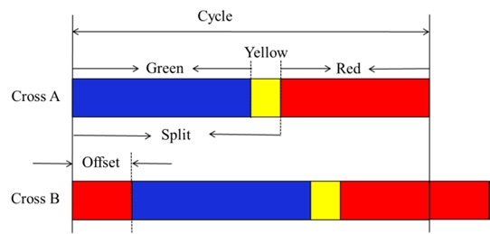
A traffic signal controls traffic by assigning right-of-way to one traffic movement or several non-conflicting traffic movements at a time. The right-of-way is assigned by tuning on a green signal for a certain length of time, or an interval. The right-of-way is ended by a yellow change interval during which the yellow signal is displayed, followed by the display of a red signal.
The parameters of traffic signal control,
The control methods of traffic signals are classified into a point control, a line control, and a wide control from the perspective of controlled objects. Wide controls and/or the line controls generally require an enormous quantity of transmission and a great deal of time. In addition, the adjustment of the parameters for traffic signals is classified into an actuated control and a pretimed control. The trafficactuated control of isolated intersections attempts to continuously adjust green-time. These adjustments occur in accordance with real-time measures of traffic demand obtained from vehicle detectors placed on one or more of the approaches to the intersection. On the other hand, the pretimed signal control assigns right-of-way at an intersection according to a predetermined schedule. The sequence of right-of-ways (splits or phases), and the length of time interval for each signal indication in cycles is fixed based on historic traffic patterns.
In the actual situation, the traffic flow is changed randomly and its randomness makes the control of traffic signals difficult. An estimation of the traffic volume is, therefore, necessary and effective for reducing traffic jams. In addition, an autonomous distributed (stand-alone) point control for individual traffic lights is better than wide and/or line controls from the perspective of real-time control.
III. STOCHASTIC CONTROL OF CROSSROADS TRAFFIC SIGNALS
>
A. Bayesian Network Stochastic Model of Traffic Flow at Crossroads
Traffic inflows and outflows at crossroads, and resulting traffic occur randomly, and their cause-and-effect relationship can be represented by a stochastic model based on a BN [24].
BN is a directed and acyclic graphical model. Each node represents the variables of given objects and their direct causal relationship is represented as an arc. The relationship between each variable is evaluated quantitatively using conditional probabilities.
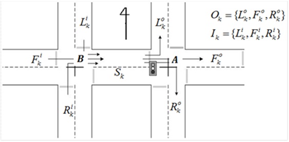
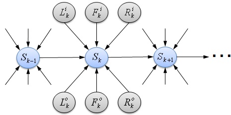
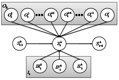
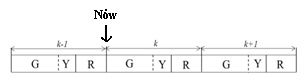
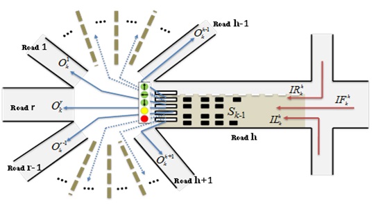
Here, we consider two crossroads as shown in Fig. 2. The random variables of traffic inflows and outflows of the crossroad, and the standing vehicles between the two crossroads are represented as nodes. The BN model of the standing vehicles is shown in Fig. 3 [25].
The number of standing vehicles of

Sk : Standing vehicles at k - th cycle
Sk-1 : Standing vehicles at (k-1) - th cycle
Fok : Outflowing straight vehicles at k - th cycle
Lo:k : Outflowing left turn vehicles at k - th cycle
Rok : Outflowing right turn vehicles at k - th cycle
Fik : Inflowing straight vehicles at k - th cycle
Lik : Inflowing left turn vehicles at k - th cycle
Rik : Inflowing right turn vehicles at k - th cycle
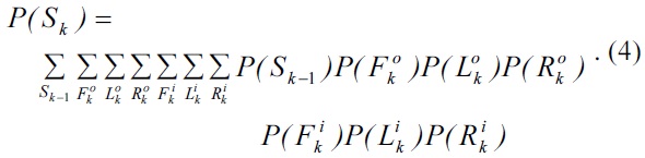
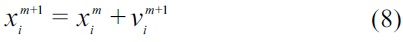
The probabilistic distribution of standing vehicles
Where
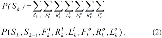
Following the chain rule, the joint probabilistic distribution is represented as the product of conditional probabilities as follows:
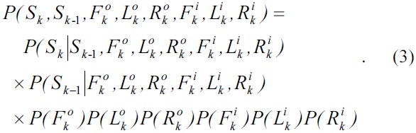
According to the D-separation [24] and the standing vehicle
However, the probabilistic distributions of the outflows
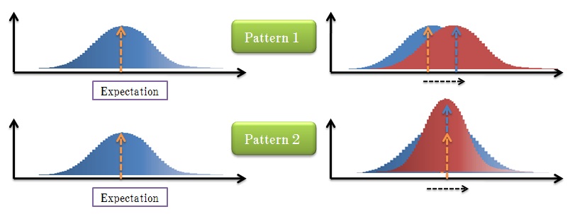
The probabilistic distributions of traffic outflows and inflows at
Pattern 1 is a shifting of the probabilistic distributions according to the fluctuation of green-time, and pattern 2 is an increase in the probability for neighboring expectation and a decrease of others (Fig. 5). Pattern 2 is adopted to update the probabilistic distributions of traffic flows based on simulations.
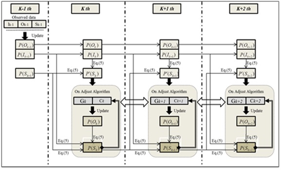
In order to deduce adequate traffic signals, the probabilistic distributions of standing vehicles are predicted to three cycles ahead as an example in this paper. The procedure of updating for prior probabilities and prediction for probabilistic distributions of standing vehicles is illustrated in Fig. 6. First, the prior probabilities of each variable are updated by previous data at cycle (
>
B. Traffic Signal Control Based on Predicted Probabilistic Distributions of Standing Vehicles
1) Rule-Based Control
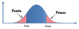
Reduction of traffic jams for a major street (e.g., the eastwest direction of Fig. 2) can be achieved by extension of green-time to reduce the probabilistic distribution of the major street. However, in this case, the probability of traffic jams for a minor street (for example, the north-south direction) will be increased by the long red time of the minor street. Therefore, the probabilities of an over-standing vehicle
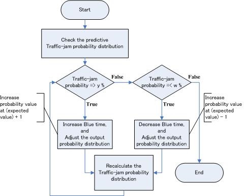
According to the BN stochastic model, the probabilistic distribution of the standing vehicle, splits, and cycle time of traffic signals are controlled by using the predicted probabilistic distributions of standing vehicles. A rule-based control procedure is as follows:
Step 1: Predict probabilistic distribution of standing vehicles by using a BN stochastic model to three cycles ahead.
Step 2: Calculate probabilities Smax or above and Smin or below of standing vehicles.
Step 3: Compare these probabilities with the desired values.
Step 4: Adjust split and cycle time until probabilities Smax or above and Smin or below satisfy the desired values.
The flowchart of the procedure for traffic signal control is shown in Fig. 8.
2) Back Propagation NN Control
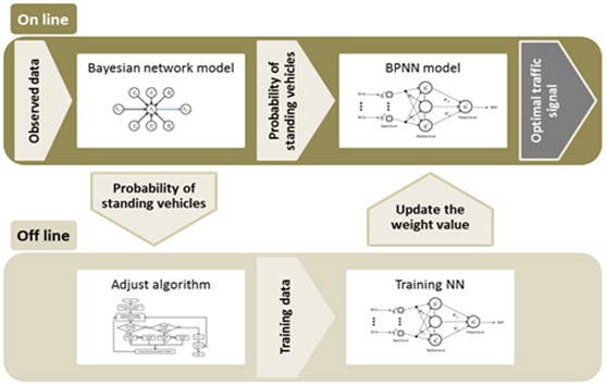
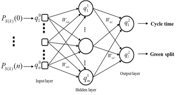
Traffic signal control is composed of two procedures: online and offline processing. In the online processing, a back propagation neural network (BPNN) is used to calculate adequate traffic signals based on the result of a BN stochastic model for the prediction of standing vehicles. Then, the rule-based algorithm is applied to update the weight of the BPNN model in the offline processing.
The BPNN model has a powerful learning capability, and this model consists of an input layer, a hidden layer, and an output layer. The BPNN model for traffic signal control is shown in Fig. 9 [26]. The input values are the probabilities of standing vehicles, which are predicted by the BN model, and the output values are traffic signals.
In this BPNN model, the number of neurons for the input layer is 141, and the inputs are the probabilities of standing vehicles. The traffic signal comprises two parameters:
The procedure of traffic signal control using the BPNN model is illustrated in Fig. 10.
>
C. Stochastic Optimum Control of Crossroads Traffic Signals
1) Formulation for Optimization of Traffic Congestion Problem
It is necessary to reduce traffic jams of a major street and a minor street both for the reduction of traffic volume at crossroads. However, when the green-time of the major street is extended to reduce the traffic jams of the major street, the traffic congestion of the minor street will be increased because the red-time of the minor street has been extended. Therefore, the traffic congestion problem at crossroads is a trade-off between the length of green-time and red-time (i.e., green-time of the minor street) for the major street. An adequate method of the reduction of traffic volume at crossroads is a prediction of probabilistic distributions of traffic jams and reduction of probabilities for over-standing vehicles and under-standing vehicles of the major street together.
As an optimization problem of traffic congestion at crossroads, a performance criterion is defined as follows [25]:
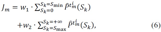
where

is a predicted probabilistic distribution of the major street when the traffic signals are
2) Construction of Traffic Flow Micro-Simulator by Cellular Automaton
The probabilistic distribution of traffic outflows is necessary to predict the probabilistic distribution of standing vehicles at
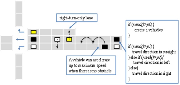
The traffic outflows are estimated by using an urban traffic flow micro-simulator based on a cellular automaton (CA), which is an example of artificial life, built based on a model of a highway [27]. The rules of vehicles movements on roads are illustrated in Fig. 11, where the parameters
Input to cell: According to the generation of a random number for an inflow rate, a vehicle is generated and the direction of travel to the next intersection is determined. The inflow rate of each road is determined by measured traffic data.
Movements: A vehicle can accelerate up to a maximum speed when a front cell is free of obstruction. Considering a mean speed in an urban area, the maximum speed is set at 2 cells/1 step (1 cell = 7.5 m; 1 step = 1 sec). According to the density of the traffic, the speed can change randomly. On multi-lane roads, vehicles can move in parallel lanes. When a vehicle turns right, the vehicle moves to a right-turn-only lane. (Following Japan’s traffic patterns, the model assumes driving on the left side of the street.)
Intersection: When a traffic signal is green, a vehicle is allowed to cross the intersection according to its direction of travel, and the direction of travel at the next intersection is reset.
3) Searching for Traffic Signals by Using the PSO Method
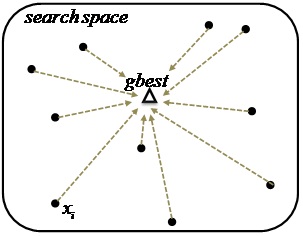
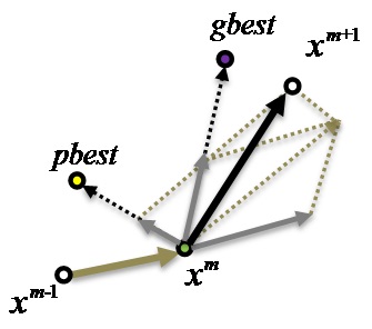
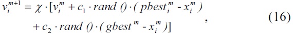
The PSO method was introduced by Kennedy and Eberhart [28]. The PSO method is based on a simple mechanism, which mimics the swarming behavior in birds flocking and fish schooling to guide particles to search for optimal solutions. The PSO method is easy to implement and use with only a few parameters to adjust. In the PSO method, a swarm of particles is represented as potential solutions and each particle is associated with a velocity vector
During the evolutionary process, the velocity and position of a particle
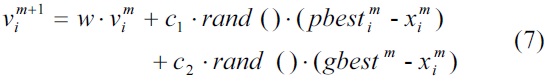
where
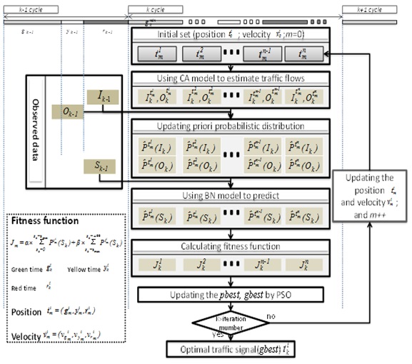
Step 1: Set the number of particles in the swarm, and an initial position and velocity of each particle. The initial position of a particle i: tio=(gio, yio, rio) represents the signal times of green, yellow, and red, respectively, and their initial times are produced randomly. Also, the initial velocity of the particle i: vio = (vgio, vyio, vrio) represents the initial updating of green, yellow, and red times, and their initial number of updates are produced randomly in [-2, +2]. Set the number of searches to m = 0.
Step 2: Estimate the traffic inflows Ik and outflow Ok of crossroads at k-th cycle by using the CA micro-simulator.
Step 3: Update the prior probabilistic distributions of traffic inflow

and outflow

at
Step 4: Predict the probabilistic distribution of traffic jam

at k-th cycle using the BN stochastic model.
Step 5: Calculate the performance criterion Jm using

Step 6: Update pbest and gbest of the PSO algorithm.
Step 7: If m < mmax: update the positions and velocities of all particles, and Go to step 2;
Else, output the positions of gbest (green - yellow - red times).
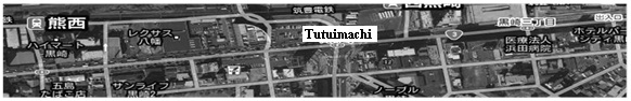
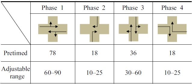
A simulation was carried out to confirm the effectiveness of stochastic control of traffic signals at crossroads using actual traffic flow data. The actual data was measured on 17 January 2008, 5:00-7:00 PM at Tutuimachi crossroads, Kitakyushu, Japan, as illustrated in Fig. 14. The traffic light of the Tutuimachi crossroads is a pretimed control, its cycle length is 150 seconds and 4 phases, and their traffic lighting times are shown in Table 1.
In addition, the set values are
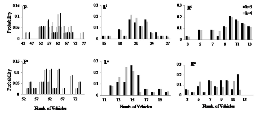
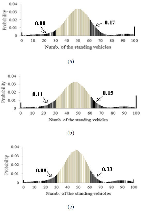
The predicted probabilistic distribution of traffic jams four cycles ahead, and the prior probabilistic distributions at Cycle 3 and the updated one at Cycle 4 of traffic inflows and outflows are shown in Figs. 15 and 16, respectively.
[Table 1.] Traffic signals of pretimed control and their adjustable range

Traffic signals of pretimed control and their adjustable range
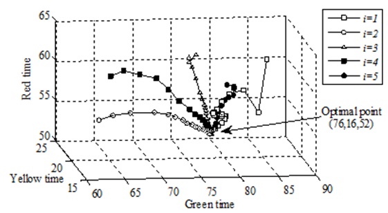
Moreover, the convergence of 5 particles (of the total 30 particles) at Cycle 4 is illustrated in Fig. 17, where the initial positions (
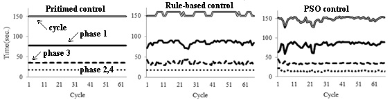
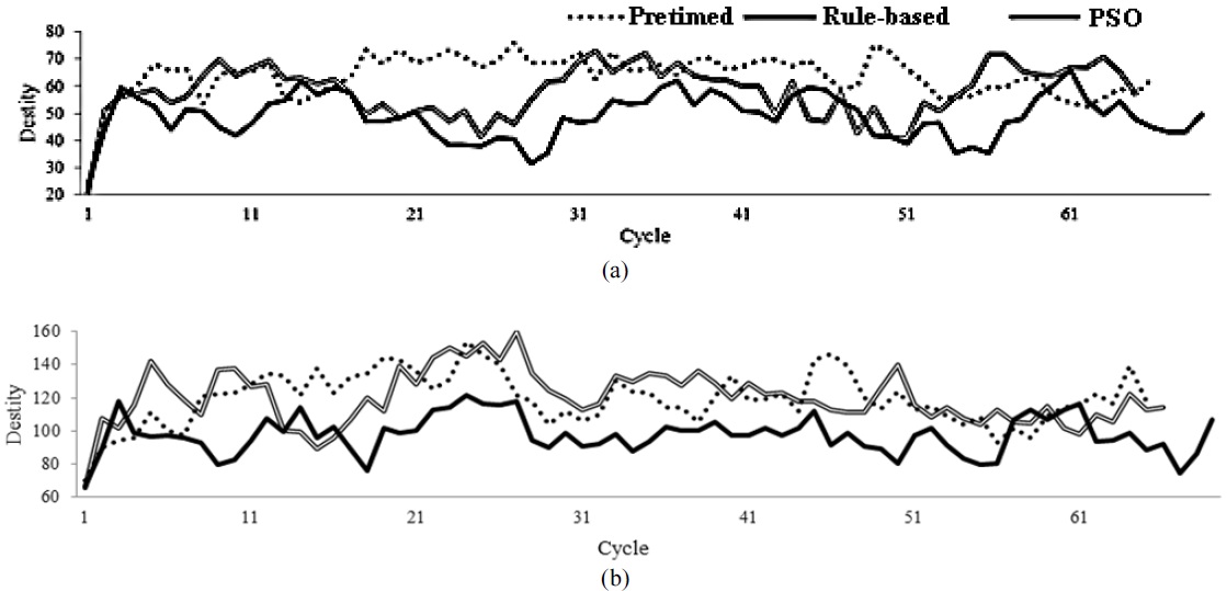
The traffic signals by pretimed, rule-based, and PSO controls and the traffic jams at crossroads are shown in Figs. 19 and 20, respectively.
The number of standing vehicles on the major street and the total number of PSO controls was reduced by 12(%) and 8(%) compared with the pretimed control, respectively.
IV. REAL-TIME STOCHASTIC OPTIMUM CONTROL OF MULTI-WAY TRAFFIC SIGNALS
>
A. Construction of BN Stochastic Model for Traffic Flow at Multi-Way Intersection
Here, we consider an
On the
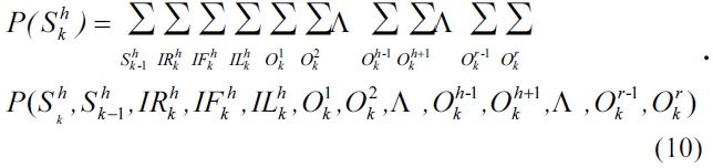
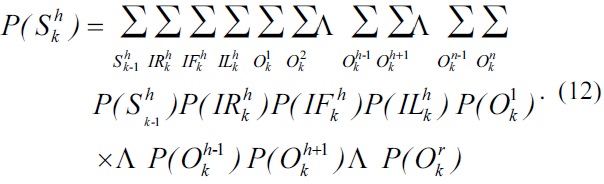
In consideration of

with the chain rule and D-separation, Eq. (10) can be represented as
>
B. Real-Time Stochastic Optimum Control of r-Way Traffic Signals
1) Formulation for Optimization of Traffic Congestion Problem at r-Way Intersection
For the
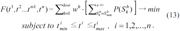
where
2) Traffic Flow Micro-Simulator by CA Model for r-Way Intersections
In order to predict the probabilistic distributions of standing vehicles, an updating rule for the prior probabilities of traffic inflows is indispensable. In this paper, Eq. (14) is used to update the prior probabilistic distributions as follows:
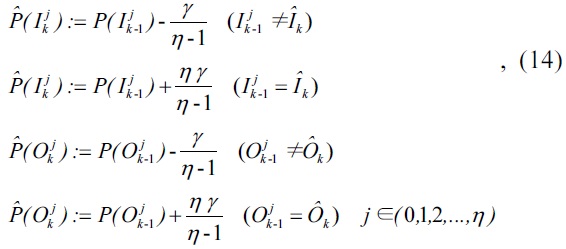
where
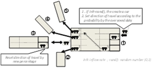
An example illustrating the rules of movements for vehicles on a road network is shown in Fig. 23.
Input to cell: A vehicle is generated and its direction of travel on the intersection is determined according to the comparison of a random number [0, 1] with a set value.
Speed: A vehicle is accelerated up to a maximum speed, where maximum speed = 2 moves/cell; 1 cell = 7.5 m/1 step (1 second), when a front cell is free of obstruction. The speed is changes randomly according to the road conditions.
Intersection: A vehicle is allowed to cross the intersection according to the direction of travel when a traffic signal is green.
Multi-lane: A vehicle can move to parallel lanes. If the direction of travel is a right-turn, the vehicle moves to a right-turn exclusive lane.
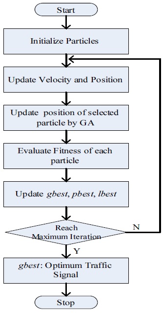
3) Search of Traffic Signals by Using the H-GA-PSO Algorithm
A fast algorithm is necessary to achieve real-time control for traffic control because the processing of the prediction and search to decide on the traffic signals of
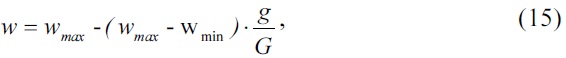
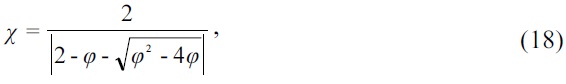
Among the modified PSO methods are the Linearly Decreasing Inertia Weight Method (LDIWM) [30] and the Constriction Factor Method (CFM) [31]. The LDIWM method makes the coefficient
These methods are expected to produce an improvement in the search; however, it is also possible for the particle to fall into a local minimum point when the particle size is small.


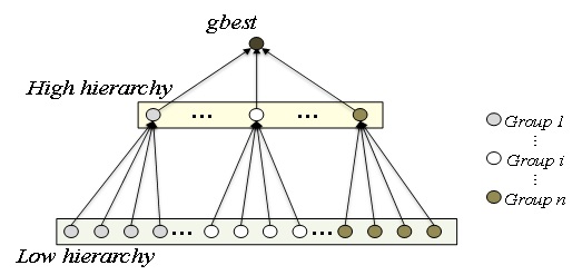
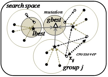
A hierarchical PSO (H-PSO, local version) method [32] can overcome this local minimum problem. The H-PSO method divides particles into several groups, and then the best particle in each group is located in a high hierarchy and the others are in a low hierarchy, illustrated in Fig. 25.
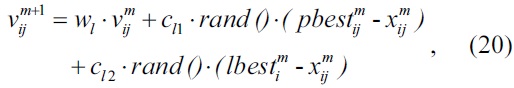

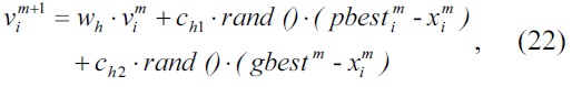

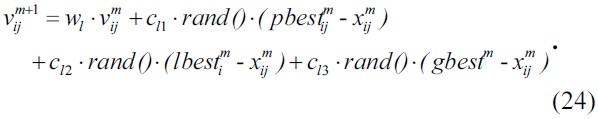
In the H-PSO method, the particles in the low hierarchy are updated using Eqs. (20) and (21), and the particles in the high hierarchy are updated using Eqs. (22) and (23), respectively. In Eq. (20),
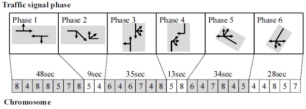
At the same time, a genetic algorithm (GA) is newly introduced to update a selected particle position to avoid the local minimum problem. The number of chromosomes is 21; one chromosome represents one cycle of the traffic signal, and one gene is an integer from 4 to 9 seconds. An example of a chromosome is illustrated in Fig. 26. Crossover processing is used to exchange two particles between two groups, and mutation processing is used to reset a particle around
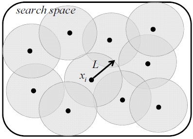
Furthermore, a rule for the initial generation of particles is newly introduced to generate the next further particle for a distance L away from a particle as illustrated in Fig. 28. The procedure for the new H-GA-PSO algorithm, which combines H-PSO with the modified velocities, GA operations, and the initial generation of particles, is shown in Fig. 29.
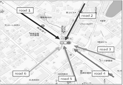
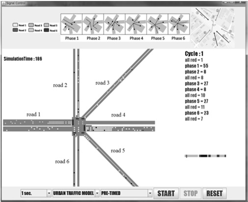
A simulation was carried out to confirm the effectiveness of the real-time stochastic optimum control of traffic signals at an
[Table 2.] Traffic signals of pretimed control at Ijiri 6-way intersection
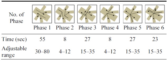
Traffic signals of pretimed control at Ijiri 6-way intersection
[Table 3.] Parameters of micro-simulator
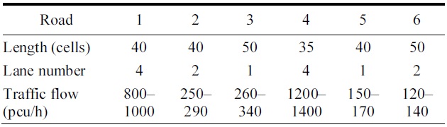
Parameters of micro-simulator
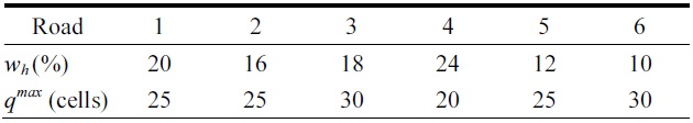
[Table 4.] Parameters of fitness function

Parameters of fitness function
In addition, the parameters of the H-GA-PSO algorithm are as follows:
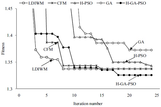
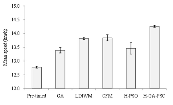
For an examination of traffic signal controls, a simulation was carried out using each of the GA, CFM, LDIWM, HPSO, and H-GA-PSO algorithms. There are three traffic congestion levels (normal, high, and very high), and their results from 20 times are shown in Table 5.
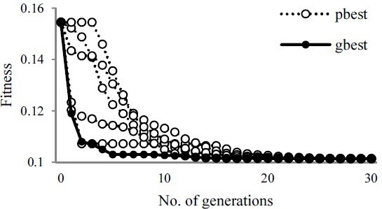
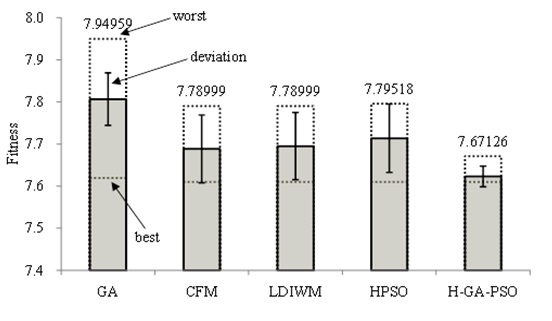
The convergence of fitness in the case of very high congestion, and the mean fitness values and their standard deviations are shown in Figs. 32 and 33, respectively.
[Table 5.] Comparison of traffic signal controls
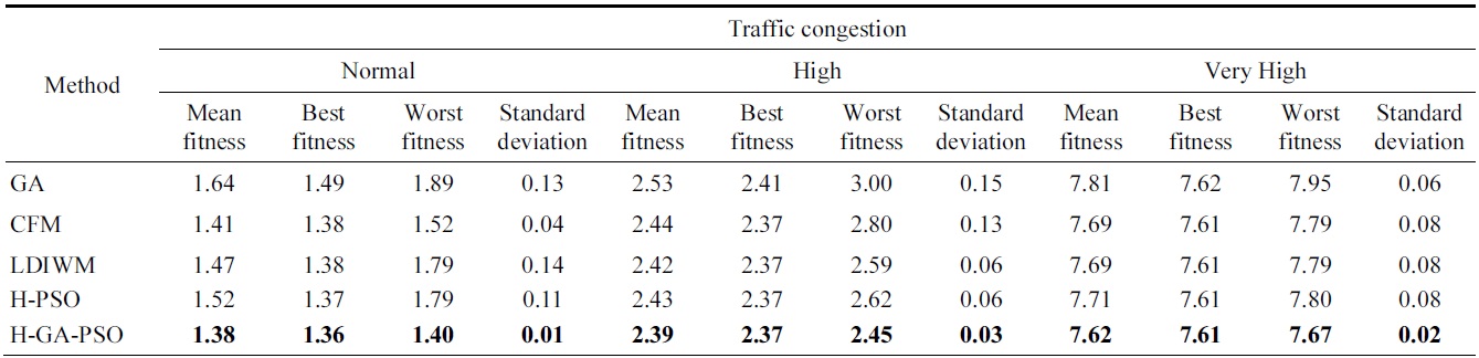
Comparison of traffic signal controls
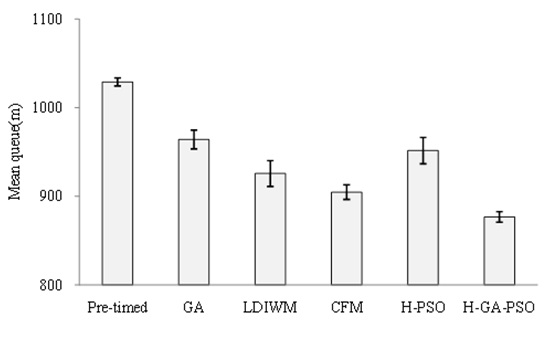
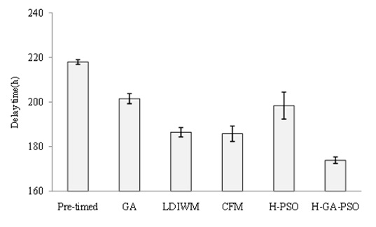
The searches by the GA and H-PSO methods do not reach the minimum value by a limited number of searches, and the searches by the LDIWM and CFM methods might fall into a local minimum point. Moreover, the mean of the traffic queue length, total delay time, and velocity are shown in Figs. 34,35, and 36, respectively.
The mean traffic queue by the H-GA-PSO control was reduced by 15 (%) compared with the pretimed control, and the total delay time was reduced by 20 (%) and 6 (%) compared with the pretimed and CFM methods, respectively. In addition, the mean velocity was accelerated 1.5% and 0.5% compared with the pretimed and CFM methods, respectively.
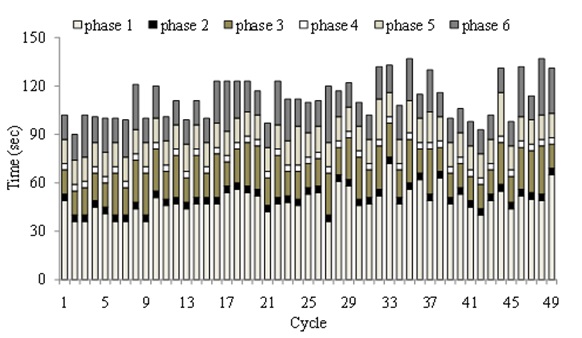
Finally, the traffic signals at Ijiri 6-way intersection of Fig. 30 by the H-GA-PSO algorithm are shown in Fig. 37.
Traffic congestion is a serious problem in modern cities, and traffic signal control is an effective method for reducing traffic jams. For actual random traffic flows, a stochastic model of traffic flows and traffic jams was constructed by using a BN, and then the probabilistic distributions of traffic jams were predicted by using a BN stochastic model and a cellular automaton model. In addition, a new H-GA-PSO algorithm was used to search for the optimum traffic signals of crossroads and multi-way intersections to realize realtime control. The effectiveness of the real-time stochastic optimum control of traffic signals was confirmed by simulations based on actual traffic data.