This paper presents a novel algorithm for nighttime detection of the lane markers painted on a road at night. First of all, the proposed algorithm uses neighborhood average filtering, 8-directional Sobel operator and thresholding segmentation based on OTSU’s to handle raw lane images taken from a digital CCD camera. Secondly, combining intensity map and gradient map, we analyze the distribution features of pixels on boundaries of lanes in the nighttime and construct 4 feature sets for these points, which are helpful to supply with sufficient data related to lane boundaries to detect lane markers much more robustly. Then, the searching method in multiple directions- horizontal, vertical and diagonal directions, is conducted to eliminate the noise points on lane boundaries. Adapted Hough transformation is utilized to obtain the feature parameters related to the lane edge. The proposed algorithm can not only significantly improve detection performance for the lane marker, but it requires less computational power. Finally, the algorithm is proved to be reliable and robust in lane detection in a nighttime scenario.
Lane detection is a well-known research field of computer vision with wide applications in autonomous vehicles and advanced driver support systems. Several researchers around the world have been developing vision-based systems for lane detection. Most of the typical systems, such as ARCADE [1], GOLD [2], and RALPH [3], present limitations in situations involving shadows, varying illumination conditions, bad conditions of road paintings and other image artifacts.
Much research on lane detection by machine vision has been carried out. As to such research, broadly speaking, the algorithms related to lane detection can be divided into two categories:
On the other hand, the model-based methods just utilize a number of parameters to represent the lanes’s boundaries. Compared with the feature-based technique, the method is much more robust against noise. Much research on modelbased lane detection has been conducted. In Ref. [8], Lakshmanan addresses the problem of locating two straight and parallel road edges in images that are acquired from a stationary millimeter-wave radar platform positioned near ground-level. In Ref. [9], Truong et al. use Non Uniform B-Spline (NUBS) interpolation method to construct the boundaries road lane. A canny filter is employed to obtain edge map and a parallel thinning algorithm is introduced to acquire the skeleton image. To estimate the parameters of lane model, the likelihood function [10], Hough transform [11], and the chi-square fitting [12], etc. are applied to the lane detection. However, most of lane models are only focused on a certain shape of lanes. Therefore, they lack the flexibility to model the arbitrary shape of road.
The proposed methods above references can detect the lane boundary or lane marker with good results under specified conditions. However, there are still some limitations, such as the failure of road recognition due to severe change of light, especially at nighttime. In details, the average gray value in images acquired in night time are notably lower than in daytime, which leads to low contrast between lane boundary (lane marker) and road background. In addition, the distribution of gray value is very nonuniform because of other influence from various light sources, for example, headlights of automobiles and street lamps. Consequently, the lane detection algorithm discussed earlier will be invalid in these conditions. Motivated by these drawbacks, a detection algorithm is introduced to recognize in nighttime the lane markers painted on the road. The algorithm studies
the imaging characteristics and analyzes distribution features of the boundary pixels in order to detect lane markers with much robustness. Combining intensity map and edge map processed by directional Sobel operator, we construct 4 feature sets for these pixels. Then, a multiple-directions searching method is conducted to suppress the false lane boundary points. Finally, adapted Hough transformation is used to obtain the feature parameters of the lane edge.
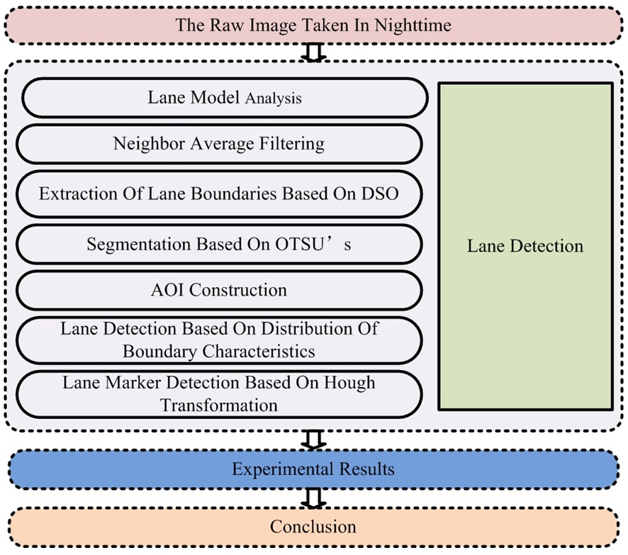
This article is organized as follows. Following the introduction, the lane detection algorithm for night-time images is presented to extract features of lane markers in Section II. Section III illustrates the lane detection results and Section IV concludes the paper. The overall algorithm flowchart is shown in Fig. 1.
The whole lane detection process is divided into 5 main steps as follows: lane modeling, image filter, image segmentation, feature extraction and parameter estimation for lane boundaries. Each of the steps will be discussed in detail in the following subsections.
2.1. Characteristics of Night Lane Images
In complicated situations where the lane is cluttered with heavy shadows or noise from other objects, the image content in various locations share similar properties with the lane boundaries.At night it becomes worse. If the feature extraction algorithm for lane detection is only allowed for a local image region, unexpected feature points of lane boundaries will be detected. These features will then be interpolated during the parameter estimation process that leads to inaccuracies and errors. Therefore, the feature points are not desired candidates and should be removed before the parameter estimation stage. And it is vitally important that we analyse characteristics of night lane images before lane detection. Compared to optics imaging in daylight, input images from a Charge-Coupled Device (CCD) in a night scenario have notably complicated characteristics as follows.
[1] The influence of other light sources. It is well known that various human-made light sources, such as street lamps, headlights, advertising lamps and so on, have been exploited in order to ensure safe driving in night due to improvement of drivers’ vision and obstacles’ visibility. However, the illumination of these light sources is much less than that of sunshine in daytime. Additionally, the intensity contrast between lane boundaries and background become much lower. It is easy to notice that the mean value of nighttime image intensity is normally so much lower that lane boundaries are blurring, which makes feature extraction more difficult.
[2] More uneven intensity distribution. Intensity distribution
of images taken from CCD in nighttime scenario is much more uneven because of a large number of external light sources. Specifically, the uneven intensity distribution that the region near the middle of nighttime images has a higher average value of intensity and the others have lower one can be observed experimentally. Furthermore, what's even worse is that several light spots or bands will be formed in a nighttime image due to illumination in different directions from light sources.
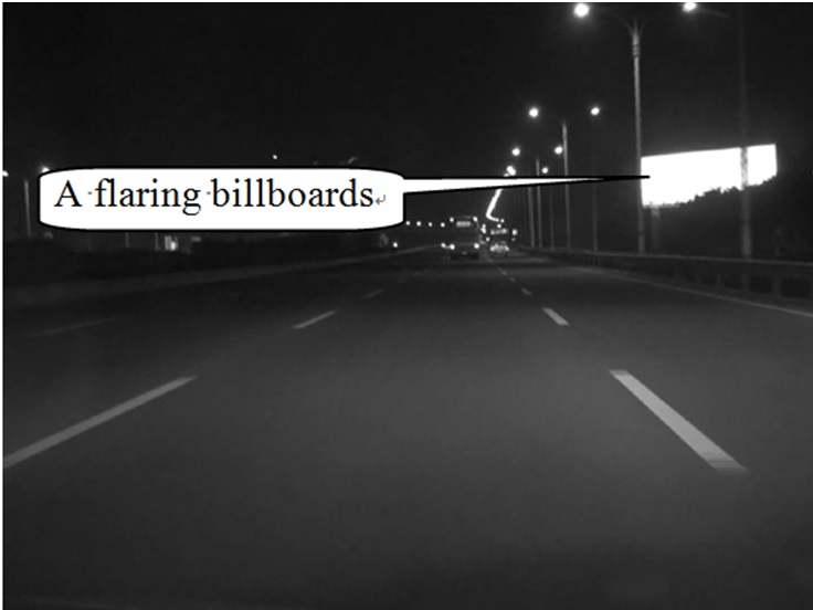
[3] The influence of billboards or traffic signs. As shown in Fig. 2, there exist large-sized billboards or traffic signs coated with reflective material or a reflective layer on either side of a lane, which leads to several large-sized light spots in nighttime images.
2.2. Analysis for Lane Modeling
So far all kinds of lane models have already been introduced, ranging from straight line segments model to fl exible splines model. However, simplified models cannot describe the lane shapes accurately, especially in the far fi eld. In another aspect, complex lane models lead to much heavier computational costs and may even increase the amount of detection error.
Actually, the imaging characteristics discussed above that inevitably introduce a large amount of noise will increase difficulty for lane detection. In order to make our proposed algorithm practical, it is necessary to define beforehand reasonable assumptions and appropriate constraints.
[1] The case that almost all pixels in the area of interest (AOI, discussed in Section II.6) are white due to light saturation is omitted in this paper.
[2] The case that almost all pixels in AOI are black because of no illumination is ignored.
[3] Lane markers are mainly painted in white or yellow with better reflective material, which distinguishes them from the background. Hence, lane markers painted on a lane have a brighter intensity level than the mean intensity of the background.
[4] To ensure safe driving at high speed, the lane generally has a much greater curvature radius in China, especially for the freeway. Accordingly, the orientation of lane markers varies smoothly along the lane. From frame to frame, the lane markers are moving backwards when a vehicle travels forward, but since the color and the width of the lane markers are similar, the driver does not feel the phenomena and considers the lane markers as static objects [13]. Additionally, the edge orientation of the lane should not be close to horizontal or vertical.
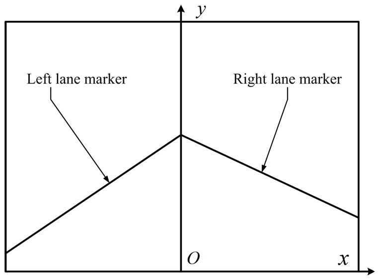
According to these assumptions, the left and right lane boundaries can be approximately regarded as a straight line in our system. The line model has been utilized most widely in the existing lane detection systems [14,15] because it combines parallel line and planar ground surface constraints, which are suitable for most of the freeway applications. In addition, the model requires lesser parameters which lead to more accurate and faster parameter estimation. Therefore, the line model for lane detection is also exploited in our work.
Assuming a flat lane, a lane image inputted from the CCD has


Where
2.3. Neighborhood Average Filtering
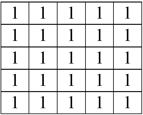
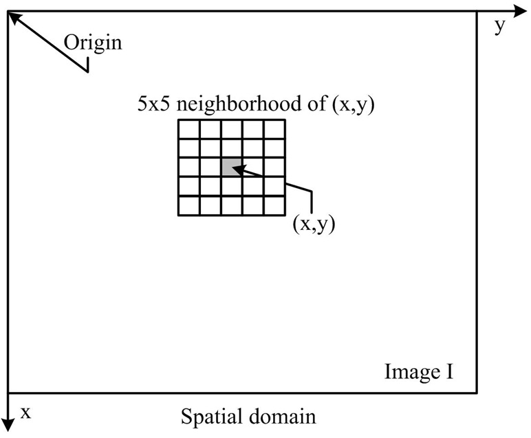
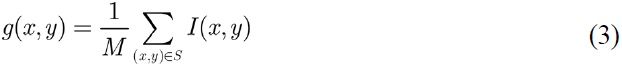
As discussed in the above section, the imaging environment at nighttime is very sophisticated with respect to image processing. There are too many negative factors making image processing difficult to apply consistently. Specifically, the uneven characteristics of illumination result in irregular light spots or light bands in nighttime lane images, where a large amount of noise is included. Furthermore, other kinds noise such as that caused by sensors, transmission channels, voltage fluctuations, quantization, etc., is extremely strong. As a result, in such a complicated imaging environments if noise cannot be effectively suppressed or even eliminated, the final results for lane detection will become inaccurate. In terms of the experimental observation, noise influence on pixels in night-time images can be treated as isolated. Hence, the intensity level of the pixels exposed to noise will be significantly different from those around them. Based on the just stated analysis, a neighborhood average filter (NAF) capable of suppressing and reducing noise has been utilized in this paper. Shown as Eq. (3),
into a spatial mask operation that is illustrated in detail in Fig. 5.
2.4. Lane Boundaries Extraction Based on Directional Sobel Operator
The subsection focuses on extracting the lane boundaries from lane background. It is generally known that edge is the most fundamental feature in an image, which widely exists between targets and background. In our work, we demonstrate the effect of the proposed algorithm operating on the feature map-
Generally, in image processing, edge is mathematically defined as the gradient of the intensity function. For an original lane image
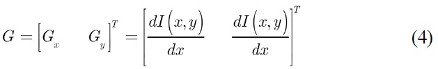
The components of the vector
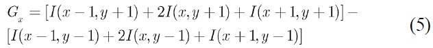
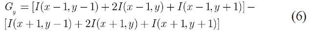
To reduce the computation of the vector

In addition, the orientation of gradient is illustrated as Eq. (8).

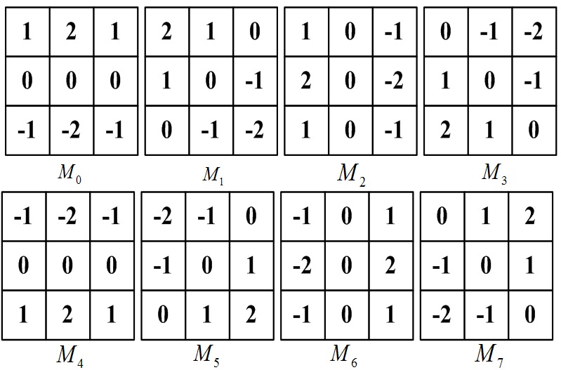
For the gradient map, based on the content mentioned in the last paragraph, we seek an effective and robust algorithm for lane boundaries extraction. Actually, many operators of edge extraction, such as Robert, Sobel, Prewitt, Laplacian, Canny operator [17] and so on, are widely utilized to pick up points on lane boundaries from cluttered background. Although the Sobel operator capable of enhancing the vertical and horizontal features of edge is one of the most classic algorithms exploited to produce gradient map for images acquired in daytime, the algorithm increases the high inaccuracy of edge extraction or even completely fails due to much more noise included in nighttime lane images. In order to address the algorithm’s failure, the directional Sobel operator (DSO) capable of highlighting the image edge feature in eight directions is introduced. It is composed of 8 spatial operators,
The experimental results of the proposed feature extraction approach based DSO and the comparison between DSO based and the other filter based feature maps can be found in Section IV.1.
2.5. Thresholding Based on Maximum Entropy
The pixels from boundaries in a nighttime lane image have a large magnitude, and they are minorities compared with other pixels. Hence, it is necessary to eliminate pixels with a smaller magnitude than a threshold value.
An image,
In our work, we use OTSU’s method, which is one of the most widely utilized thresholding technologies in image analysis. It has showed great success in image enhancement and segmentation [18]. As demonstrated in [19], it is an automatic thresholding strategy; we exploit the automatic capability for designing the unsupervised classification strategy justifying its choice.
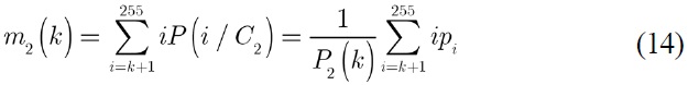
Let {0,1,2,…,255} set denote 256 distinct intensity levels in lane image of size
The normalized histogram has components
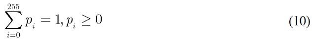
Where
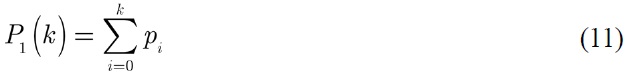
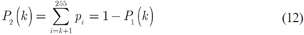
Similarly, the probability distribution of class
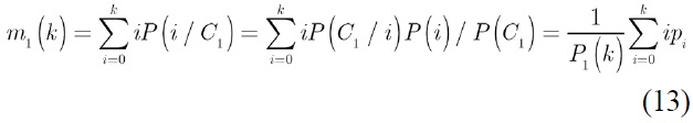
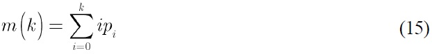
The mean intensity value of the pixel assigned to class
Similarly, the mean intensity value of the pixel assigned to class
The cumulative mean up to level
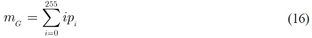
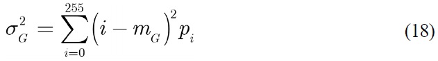
And the average intensity of the entire image is given by
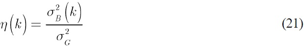
In order to evaluate the ‘goodness’ of the threshold at level
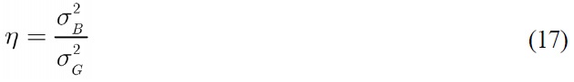
Where
And

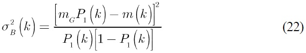
Eq. (19) can be rewritten also as Eq. (20).
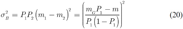
Reintroducing
and
Then the optimum threshold is the value,
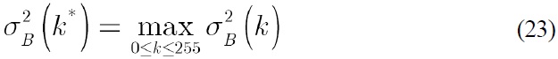
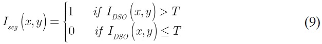
Subsequently, once the value,
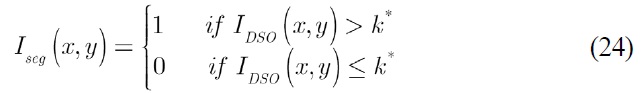
Finally, after the thesholding stated above, most of the unexpected feature points of lane boundaries are excluded from cluttering background and the rest of the feature points are labeled with ‘1’s.
This section focuses on reducing the computational costs using techniques based on area of interest (AOI). Also, this will compensate for the extra computation that the feature extraction based on DSO introduces.
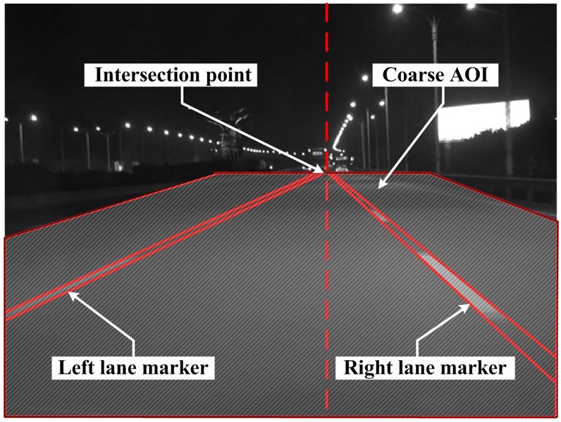
In our work, we install a digital CCD on a test vehicle. The optical axis of the CCD coincides with the centerline of the car body. Meanwhile, roll and tilt angles of installment for CCD are close to 0 degrees. Obviously, the intersection point of two lane boundaries presents in the center of the vertical direction. Now that visible lane boundaries generally lie in the lower part of an image, it is reasonable to restrict the processing area below the intersection point of two lane boundaries. In addition, assume that no horizontal or vertical lane boundaries appear in night-time lane images.
Actually, due to the deliberate installation requirements of CCD, the AOI techniques composed of the coarse AOI (C-AOI) and refined AOI (R-AOI) are realized. Specifically, we design the C-AOI for lane boundaries detection within the gray areas as shown in Fig. 7. By construction of C-AOI, we successfully make a reduction in searching time for feature extraction and sharply improve the robustness of lane location in nighttime images.
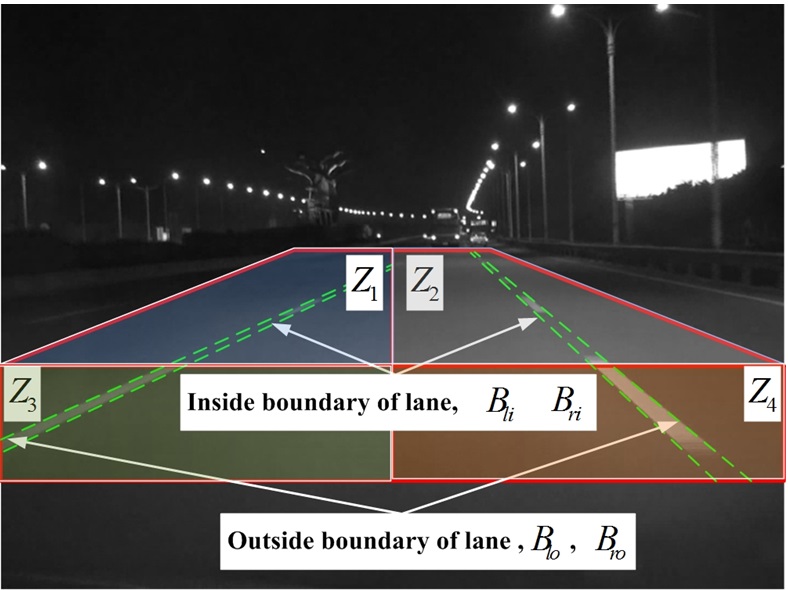
On the other hand, the R-AOI is built up in order to further suppress the influence of too much noise due to uneven illumination from various light sources and reduce the computational power. The R-AOI is composed of 4 searching regions,
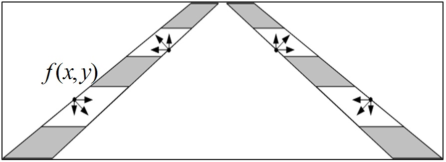
Since an important observation is that there are inside
and outside boundaries in terms of any lane marker as shown in Fig. 9, 4 sets of boundary feature,
2.7. Lane Detection Based on Distribution of Boundaries Characteristics
So far we have completed the preprocessing for lane detection, and construction of AOI and the boundaries set, which plays a significant role in lane recognition. However, how to explicitly detect lane boundaries from background and precisely describe the lane features detected with parametrization are yet unmentioned. Accordingly, it is vitally helpful, in fact, to analyse how pixels in or on boundaries distribute. In this section, we propose a processing method based on distribution features of boundaries’s pixels.
If the current pixel is
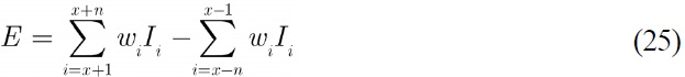
Where
[1] For the lane boundary pixels on the left plane:
A. if E ≥ Cx ? Gx > 0 ? Gy > 0 then I ∈ Blo.
B. if -E ≥ Cx ? Gx < 0 ? Gy < 0 then I ∈ Bli.
[2] For the road boundary pixels on the right plane:
A. if E ≥ Cx ? Sx > 0 ? Sy < 0 then I ∈ Bri.
A. if -E ≥ Cx ? Sx < 0 ? Sy > 0 then f(x, y) ∈ Bro.
Further experiments indicate that a possible candidate on lane boundaries may be still misclassified by the method stated above, which leads to false boundary points and even failure to detect lane. To address the misjudgment and improve the robustness of boundaries searching, an algorithm, called multi-directions searching, is performed. For example, assuming that an arbitrary pixel,
boundary sets
2.8. Lane Marker Detection Based on Hough Transformation
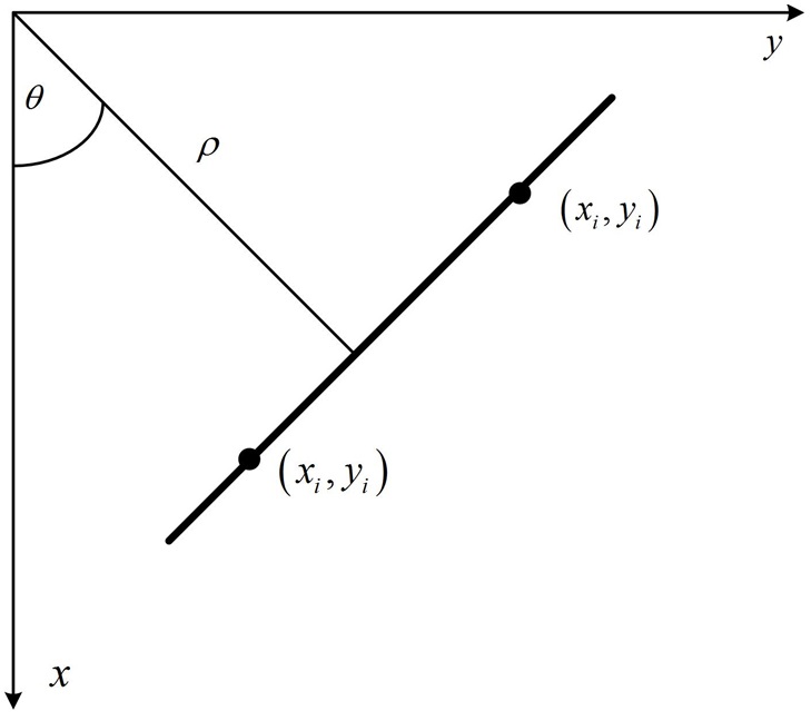
After feature extraction, the lane model parameters require to be optimised to generate an accurate representation of the lane boundaries. Finally, the results detected are then characterised by a few mathematical model parameters. In our work, the parameter optimisation stage applies the Hough Transformation (HT) [20,21], widely implemented in the other lane detection system. Given boundary points in a lane image, we expect to find the subsets of these pixels that lie on straight lines. One possible method is to search all lines determined by every pair of points and then find all subsets of points that are close to particular lines. However, this is a computationally prohibitive task in all but the most trivial applications. Suppose a boundary point (

Where (
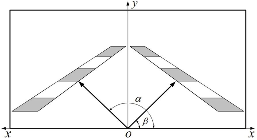
Firstly, the coordinate system is established. We divide the R-AOI into left and right region, fix the origin on the center of the bottom line and construct the two coordinate systems as shown in Fig. 11. (
using the equation
In order to enhance computational efficiency, the searching constraints are given as follows.
[1] Left lane boundary lies in the left half-plane of a lane image, and the right lane occupies the right half-plane. Therefore, left and right lane boundaries are respectively sought in the corresponding half-plane.
[2] Since the edge orientation should not be close to horizontal or vertical, as illustrated in Fig. 11, the angle between left lane boundary and χ-axis is α . Similarly, the angle between right lane boundary and χ-axis is defined as β. The calculation ranges of the two parameters, α and β, are restricted to 90°∼180° and 0°∼90°, respectively.
[3] The Eu. (26) is exploited to each pixel in the boundaries sets Blo, Bli, Bro and Bri, and obtains 4 accumulator values, Alo, Ali, Aro and Ari, corresponding to the 4 boundaries sets.
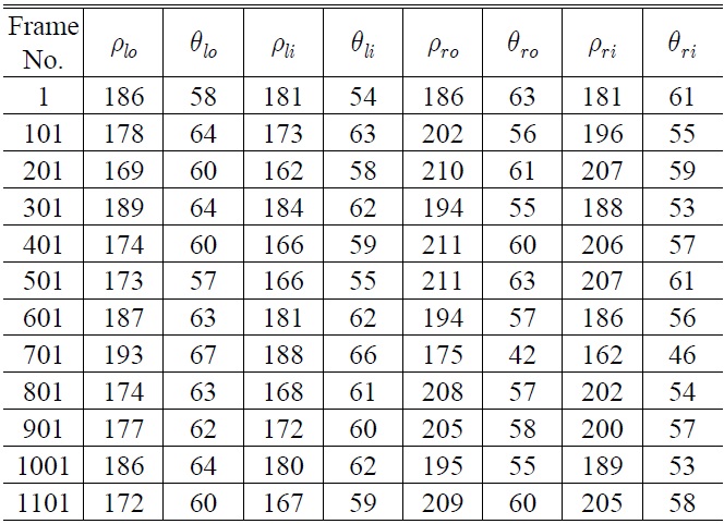
[4] To further reduce computational capacity and and enhance computational velocity, we begin to search the boundary points down from the 1 / 3 height of lane images. By selecting a cell from local maxima statistics for lane boundaries, we obtain the feature vector with 8 parameters, (ρli, θli, ρlo, θlo, ρri, θri, ρro, θro)T, in which the meanings of subscripts are identical to the definition discussed in subsection 2.6
The algorithm of lane detection was tested with images acquired by a digital CCD installed on an experimental vehicle. Experiments of lane detection were performed on highways paved with asphalt and cement while the experimental vehicle drives at a velocity around 80 km/h. Meanwhile, tests in laboratory are also conducted by recording the video sequences of the nighttime lane scenario. The image size is 320×240 (pixels). The development platform is Windows XP operation system with an Intel Pentium4 3 GHz CPU, 2 G RAM.
3.1. Lane Feature Extraction Results
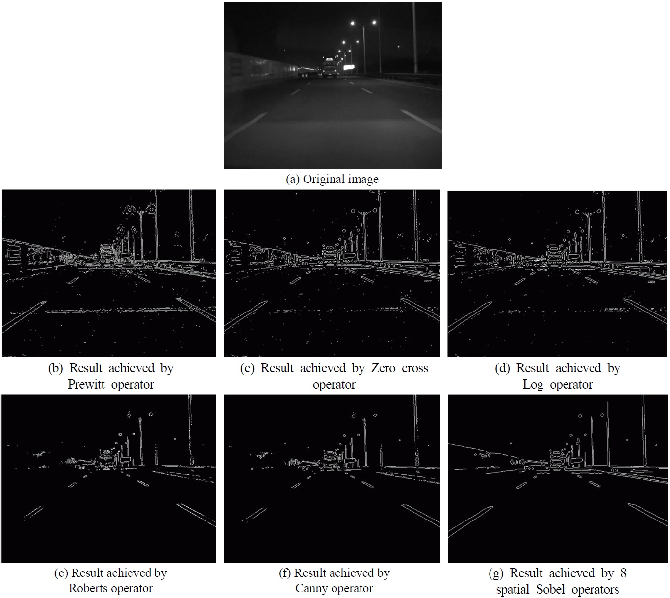
The feature extraction performance of our proposed algorithm is compared with the other traditional methods based on spatial operators, for instance Prewitt, Zero-cross, Log and so on, by which we are capable of obtaining various types of gradient maps. Some example feature extraction results are shown in Fig. 12. As the figures demonstrate, results of feature extraction acquired by using Prewitt, Zero-cross and Log operators include numerous unwanted feature points (as shown in Fig. 12(b), (c) and (d)). And it has been found that results achieved by Roberts and Canny operators can effectively extract lane features. However, they remove too much edge information that is useful for lane detection (as shown in Fig. 12(e) and (f)). Comparing these results with 8 spatial Sobel operators, significant improvement can be observed since it reserves the edge information as much as possible and includes fewer unwanted features (as shown in Fig. 12g).
3.2. Lane Feature Extraction for Multi-images
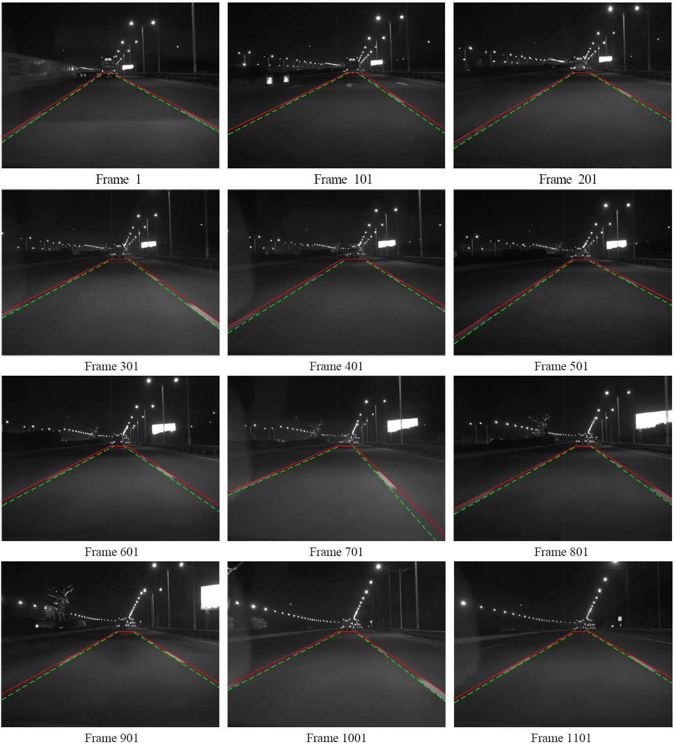
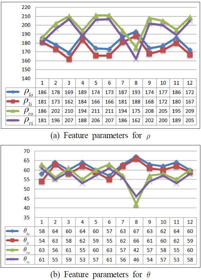
Figure 13 shows the results of 12 successive images, and Fig. 14 provides the feature parameters corresponding to the images detected. Lane representation based on a line
model is illustrated in Fig. 15, where Fig. 15(a) is for distance
and produce high quality output.
A lane detection algorithm is presented in this article. One of the significant contributions lie in the proposed lane feature extraction algorithm. Lane boundaries are modeled with straight line and neighbor average filtering is used to suppress the influence of noise in lane image taken from digital CCD. According to the discussion mentioned in preceding sections, the results of lane detection for nighttime images are good. The algorithm based on multi-directions Sobel operator is conducted to improve feature extraction of the lane edge. One of the most important results is to extract lane features based on the distribution feature of boundary points. It is capable of enhancing most of the existing feature maps by removing the irrelevant feature pixels produced by unwanted objects and sorting the extracted pixels into 4 sets of boundaries of lane, which supply sufficient data related to lane boundaries to recognize lane markers more robustly. We showed the successful results of the proposed algorithm with some real images at nighttime.