검색 전체 메뉴
PDF
맨 위로
OA 학술지
Polarization Properties of Quasi-Homogeneous Beams Propagating in Oceanic Turbulence
  • 비영리 CC BY-NC
  • 비영리 CC BY-NC
ABSTRACT

Based on the extended Huygens-Fresnel principle and generalized Stokes theory, the evolution of polarization properties of beams generated by quasi-homogenous (QH) sources propagating in clear oceanic water was studied by the use of the oceanic turbulence spatial spectrum function. The results show that the beams have similar polarization self-reconstructed behavior under different turbulence conditions in the far field, but if the propagation distance is not long enough, the degree of polarization (DOP) fluctuates with much more complexity than state of polarization (SOP) of QH beams. The self-reconstructed ability of DOP at the special distance in turbulence would get to the best value if the values of coherence of width were chosen suitably, but for SOP, it has no best value.


KEYWORD
Quasi-Homogenous source , Oceanic turbulence , Polarization self reconstruction
  • I. INTRODUCTION

    The QH beams which can be generated by SLMs have been studied and used widely in recent years [1]. The coherence and polarization properties of quasi-homogenous sources in the far field has been studied by Korotokva [2]. The coherence of properties of the field generated by a beam radiated from a quasi-homogenous electromagnetic source scattering on QH media has been studied by Xin [3]. Chen and Li have been researched the coherence properties and polarization modulation of QH beams scattered from anisotropic media [4-5]. The propagation properties of laser beams in random media like turbulence or human tissue are important for applications such as optical imaging, remote sensing and communication systems so more and more researchers are attracted [6-11]. The polarization “self-reconstructed” phenomenon in atmosphere turbulence has been known for a long time. The normalized spectrum of the beam generated by QH source after propagating through turbulent media has been proved to be equal to the normalized spectrum of the source [12]. The degree of polarization of electromagnetic Gaussian-Schell beams and partially coherent electromagnetic flat-topped beams also have self-reconstructed properties in atmospheric turbulence [13-14]. However, recent reports have shown that beams generated from anisotropic sources don’t have polarization self-reconstructed properties in turbulent media [15-16]. On the other hand, oceanic turbulence is an important natural random medium but the light propagation though oceanic turbulence is a relatively unexplored topic compared to that in other media. The spatial spectrum model of oceanic turbulence combining temperature and salinity fluctuations is only used by a few articles to study the light propagation in the oceanic waters [16-18].

    In this paper, we focused on the polarization features of QH beams propagating through oceanic turbulence. The analytical expressions of on-axis generalized Stokes parameters of QH beams were calculated,then the variations of DOP and SOP of QH beams traveling through oceanic turbulence have been simulated. The self-reconstructed properties of such beams in the far field in turbulent media have been analyzed under different source parameters and turbulence conditions.

    II. METHODS

    For beams generated by quasi-homogenous (QH) sources the spectral density S(0)(r) varies much more slowly with position vector than the correlation coefficients μij(0)(r,ω) change with difference of position vector r1-r2. The cross spectral density matrix of QH sources can be expressed as:

    image

    The superscript (0) denotes quantity pertaining to the incident field. The spectral density can be expressed as the trace of cross spectral density matrix:

    image

    (r1,r2,ω), aij(ω) is the frequency dependent factor which connects the spectral components: Sy(0)(ω)=α (ω)Sχ(0)(ω).

    image

    For α =0, the source generated linearly polarized light in the x direction, for α →∞, the light is linearly polarized in the y direction. Without loss of generality, the spectral density and correlation coefficients can be described by the Gaussian-Schell model:

    image
    image

    A is spectral amplitude which we set A=1 in this article, and Bij is called the coefficient of correlation between the incident field components, for quasi-homogenous beams, it can be set as: Bxx=Byy=1, Bxy=B*yx, where the asterisk means complex conjugate. σ represents the width of the source, δij represents the coherent width of the source. Several conditions of the source must be satisfied in order to produce a physically reliable QH beam [19].

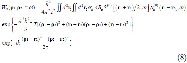
    The cross spectral density matrix of the beam at the receiving plane can be derived by the extended Huygens- Fresnel principle:

    image

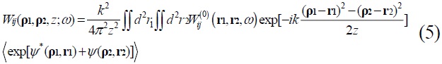
    Where r1, r2 are two arbitrary position vectors of points on the source plane while ρ1, ρ2 are two position vectors of observation points on the receiving plane. z is propagation distance and

    image

    is the wave number of the beam. The last term in Eq. (5) represents the correlation function of the complex phase perturbed by random media:
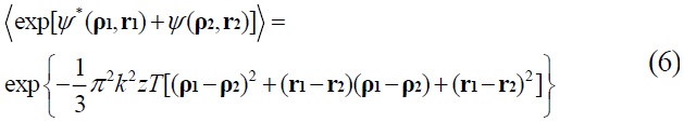
    image

    Where

    image

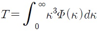
    describes the strength of turbulence perturbation.

    The model of the spatial power spectrum of refractive index fluctuations of homogenous and isotropic oceanic turbulence can be described as a linearly polynomial of temperature fluctuations and salinity fluctuations:
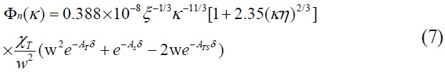
    image

    In Eq. (7), ξ is the rate of dissipation of kinetic energy per unit mass of fluid, ranging from 10-4m2s-3 in turbulence surface layer to 10-10m2s-3 in the mid-water column. χT is the rate of dissipation of mean squared temperature ranges from 10-2K2s-1 below the oceanic turbulence to 10-10K2s-1 at the mid-water column. η is the Kolmogorov micro scale. Other parameters in Eq. (7) are:

    AT = 1.863×10⁻², AS = 1.9×10⁻⁴, ATS =9.41×10⁻³, δ = 8.284(κη)4/3 + 12.978(κη)2 ; w defines the ratio of temperature to salinity contributions to refractive index spectrum which in oceanic waters varies in the interval [-5;0], with -5 and 0 corresponding to dominating temperature-induced and salinityinduced optical turbulence, respectively.

    From Eq. (3)-Eq. (6), the cross spectral density matrix of the electromagnetic field on the receiving plane can be expressed as:

    image

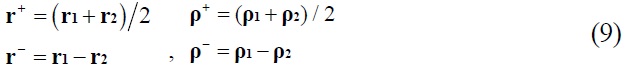
    As a matter of convenience, we make changes of the spatial arguments:

    image

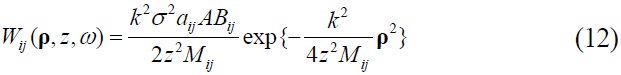
    With the help of Eq. (9), the cross spectral density matrix on the receiving plane is derived:
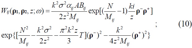
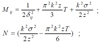
    image

    Where

    image

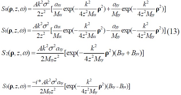
    The polarization properties of an electromagnetic beam at a point in space can be determined by use of Stokes parameters which have recently been generalized from one-point quantities to two-point counterparts [20]. They contain not only polarization properties but also coherence properties of beams [21] and can be measured by Young’s interference experiment [22-23]. The changes of generalized Stokes parameters in optical system or random media are also interesting problems and have received a lot of attention [24-25]. The four parameters can be expressed as follows:

    image

    where

    image

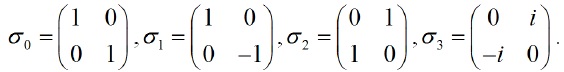
    are Pauli spin matrices:

    image
    image

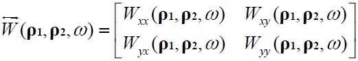
    represents the cross-spectral density matrix (CSDM) of the beam:

    image

    If we only considered polarization properties of one point, i.e., ρ1=ρ2=ρ, From Eq. (10), each element of the CSDM can be derived as the expression of:

    image

    Inserting Eq. (11) into Eq. (12), and using the conditions of Mxy=Myx, αxy=αyx the analytical expressions of four Stokes parameters can be obtained:

    image

    The polarization properties can be expressed as the functions of these four parameters.

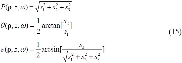
    We considered the degree of polarization and the state of polarization of QH beams in this paper. DOP is used to describe the polarized portion of a beam. DOP=1 means perfectly polarized beam while DOP=0 means unpolarized beam. The state of polarization (SOP) includes the azimuth angle and ellipticity. The azimuth angle θ is defined by the smallest angle formed by the positive x-direction and the direction of major semi-axis of the ellipse. ε , which determines the shape of the ellipse, is the ratio of the major semi-axis and the minor semi-axis.

    For convenient, we normalized three Stokes parameters by S0 as:

    image

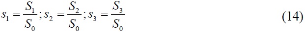
    The DOP and SOP can be expressed as the function of normalized Stokes parameters:

    image

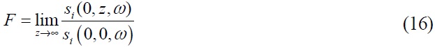
    Because of the uniform polarization properties of quasihomogenous beams, we only need to consider the on-axis point of the beam. And in order to prove the polarization self-reconstructed properties of QH beam, we should study far-field polarization properties of normalized Stokes parameters. First, let’s consider the limit as follow:

    image

    Where si(0, z, ω) are normalized Stokes parameters on the receiving plane while si(0, 0, ω) are such parameters on the source plane. From Eq. (13),

    image

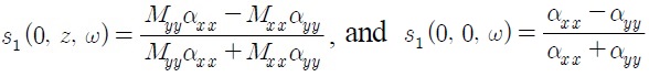
    can be obtained from Eq. (1) - Eq. (4). Then substituting into the limit of the ratio of two parameters, we get:

    image

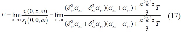
    In turbulent medium,
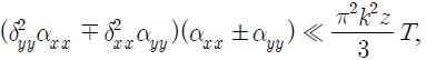
    image

    so F=1, then we proved the self-reconstructed property of s1. Other parameters in Eq. (14) can also be proved similarly, then DOP and SOP self-reconstructed properties can be derived directly. We set follow parameters to judge the ability of the self -reconstructed property of QH beams:

    image

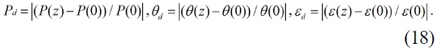
    These parameters are modulus values of relative difference of the on-axis DOP and SOP between the source plane and the receiving plane at a special distance z in turbulences, the self-reconstructed ability will be better when these values get closer to 0.

    III. RESULTS

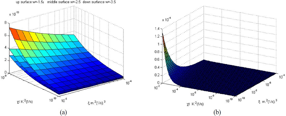
    Figure 1 shows the strength of oceanic turbulence changes with turbulence parameters: w, χT and ξ . It can be easily found out that the strength of turbulence T increases with the increase of χT and w, but reduces with the increases of ξ.

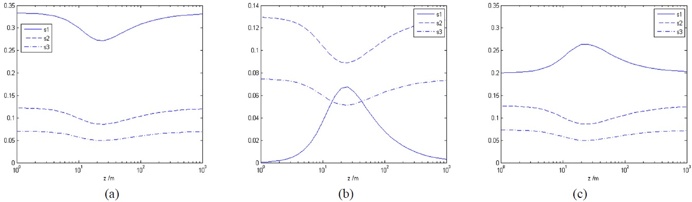
    Figure 2 shows the changes of normalized Stokes parameters with distance at different a. The DOP and SOP we calculated in Eq. (17) and Eq. (19) could be expressed as the function of these parameters, so the behavior of generalized Stokes parameters decides the evolution of DOP and SOP of the beam through propagation.

    In Fig. 3, we illustrated how the DOP and SOP of the QH beams depend on the parameters of oceanic turbulence. The effect of w on the changes of DOP and SOP has been shown in Fig. 3(a1)-(a3) and the effect of χT and ξ has been shown in Fig. 3(b1)-(b3).

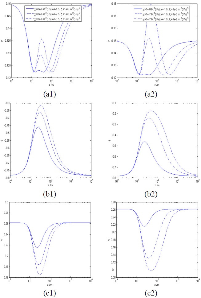
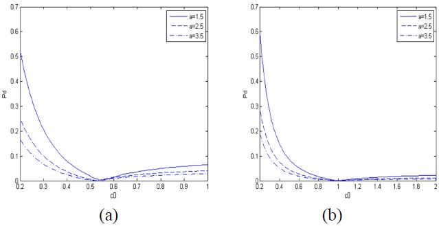
    In Fig. 4, the influence of coherent width and the coefficients αij(ω) on the changes of self-reconstructed properties of DOP of QH beams were revealed. While δyy and δxx are kept fixed, c0 is the coefficient to decide the value of δxx as the form δxx = c0δxy.

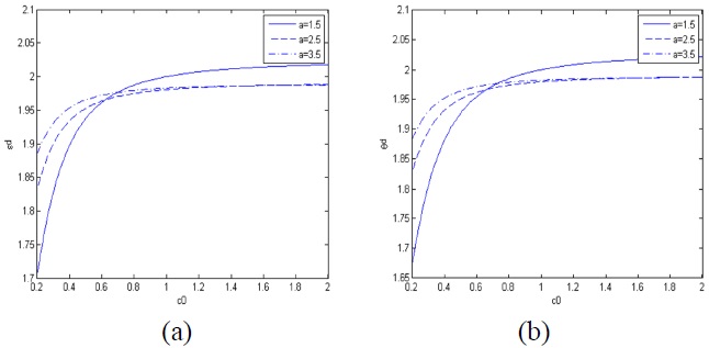
    In Fig. 5, the self-reconstructed behavior of azimuth angle θ and the degree of ellipticity ε were judged as the same method of DOP we plotted their variation versus c0.

    IV. DISCUSSION

    (1) Both DOP and SOP fluctuate at the range of 0.01 km1 km. DOP and SOP get more fluctuations in weak turbulence and get larger self-reconstructed distance than that in strong turbulence.

    (2) S2 and S3 in ocean waters fluctuate less than S1 during the propagation but they will all reach the initial value if the propagation distance is long enough.

    (3) DOP varies with more complexity with distance in ocean waters than SOP. The self-reconstructed distance of both decreases with the increase of χt and w, but increases with the increases of ξ .

    (4) When δyy=δxy, Pd reaches the minimum value, and it’s almost equivalent for different α ,but if δxxδxy, as what have shown in Fig. 4(b), Pd will get to minimum value at different c0 for different α.

    (5) εd and θd increase as increases but will change slowly when c0>1. It means when other parameters are kept fixed, the coherence width δxx should be controlled to be smaller than δxy in order to obtain better SOP self-reconstructed properties, but these two variables of SOP have no minimum values with the variation of c0.

    V. CONCLUSION

    According to our analysis, the normalized Stokes parameters will be affected by temperature and salinity fluctuations so the DOP and SOP will also be affected. And s1 fluctuates much more than s3 and s3, DOP varies with more complexity than SOP. Furthermore, both of normalized generalized Stokes parameters of QH beams have proved to be equal to the initial value if the propagation distance is long enough, so the self-reconstructed properties of DOP and SOP of such beams can also be proved. The choice of coherence width of the QH beams can help us to get the best self-reconstructed ability of DOP, but for two parameters of SOP, there are no best choices of these parameters. Our work may be helpful to develop underwater optical imaging or communication system.

참고문헌
  • 1. Mandel L., Wolf E. 1995 Optical Coherence and Quantum Optics google
  • 2. Korotkova O., Hoover B. G., Gamiz V. L., Wolf E. (2005) “Coherence and polarization properties of far fields generated by quasi-homogeneous planar electromagnetic sources” [J. Opt. Soc. Am. A] Vol.22 P.2547-2556 google cross ref
  • 3. Xin Y., Chen Y., Zhao Q. (2007) “Changes of spectrum of light scattering on quasi-homogenous random media” [Proc. SPIE] Vol.6786 P.67864S-1-67864S-9 google
  • 4. Chen J., Chen F., Chen Y. (2012) “Coherence properties of the scattered electromagnetic field generated by anisotropic quasi-homogeneous media” [Opt. Commun.] Vol.285 P.3955-3960 google cross ref
  • 5. Li J., Shi Z., Ren H. (2012) “Polarization modulation of electromagnetic waves scattered from a quasi-homogeneous anisotropic medium” [IOP Science] P.125705-1-125705-6 google
  • 6. Kwon K., Son T., Yeo C., Jung B. (2011) “Numerical modeling of compression-controlled low-level laser probe for increasing photo density in soft tissue” [J. Opt. Soc. Korea] Vol.15 P.321-328 google cross ref
  • 7. Shu Z.-f., Dou X.-k., Xia H.-y., Sun D., Han Y., Cha H., Kim D., Wang G.-c., Baik S., Hu D.-d. (2012) “Low stratospheric wind measurement using mobile rayleigh doppler wind LIDAR” [J. Opt. Soc. Korea] Vol.16 P.141-144 google cross ref
  • 8. Lee J. H., Jung Y.-S., Ryoo S.-Y., Kim Y.-J., Park B.-U., Kim H.-J., Youn S.-K., Park K.-W., Lee H. B. (2011) “Imaging performance analysis of an EO/IR dual band airborne camera” [J. Opt. Soc. Korea] Vol.15 P.174-181 google cross ref
  • 9. Gao W. (2006) “Changes of polarization of light beams on propagation through tissue” [Opt. Commun] Vol.260 P.749-754 google cross ref
  • 10. Gao W., Korotokova O. (2007) “Changes in the state of polarization of a random electromagnetic beam propagating through tissue” [Opt. Commun.] Vol.270 P.474-478 google cross ref
  • 11. Ricklin J. C., Davidson F. M. (2002) “Atmospheric turbulence effects on a partially coherent Gaussian beam: implications for free-space laser communication” [J. Opt. Soc. Am. A] Vol.19 P.1794-1802 google cross ref
  • 12. Salem M., Korotkova O., Dogariu A. (2004) “Polarization changes in partially coherent electromagnetic beams propagating through turbulent atmosphere” [Waves Random Media] Vol.14 P.513-523 google cross ref
  • 13. Roychowdhury H., Wolf E. (2004) “Invariance of spectrum of light generated by a class of quasi-homogenous sources on propagation through turbulence” [Opt. Commun.] Vol.241 P.11-15 google cross ref
  • 14. Kashani F. D., Alavinejad M., Ghafary B. (2009) “Polarization characteristics of aberrated partially coherent flat-topped beam propagating through turbulent atmosphere” [Opt. Commun.] Vol.282 P.4029-4034 google cross ref
  • 15. Du X., Zhao D., Korotkva O. (2007) “Changes in the statistical properties of stochastic anisotropic electromagnetic beams on propagation in the turbulence” [Opt. Express] Vol.25 P.16913-16915 google
  • 16. Zhou Y., Huang K., Zhao D. (2012) “Changes in the statistical properties of stochastic anisotropic electromagnetic beams propagating through the oceanic turbulence” [Appl. Phys. B] Vol.109 P.289-294 google cross ref
  • 17. Korotkova O., Farwell N. (2011) “Effect of oceanic turbulence on polarization of stochastic beams” [Opt. Commun.] Vol.284 P.1740-1746 google cross ref
  • 18. Lu W., Liu L., Sun J. (2006) “Influence of temperature and salinity fluctuations on propagation behavior of partially coherent beams in oceanic turbulence” [J. Opt. A: Pure Appl. Opt.] Vol.8 P.1052-1058 google cross ref
  • 19. Korotkova O., Salem M., Dogariu A., Wolf E. (2004) “Beam conditions of radiation generated by an electromagnetic Gaussian Schell-model source” [Opt. Lett.] Vol.29 P.1173-1175 google cross ref
  • 20. Korotkova O., Wolf E. (2005) “Generalized Stokes parameters of random electromagnetic beams” [Opt. Lett.] Vol.30 P.198-200 google cross ref
  • 21. Tervo J., Setala T., Roueff A. (2009) “Twp-point stokes parameters: interpretation and properties” [Opt. Lett.] Vol.34 P.3074-3076 google cross ref
  • 22. Kanseri B., Kandpal H. C. (2010) “Experimental determination of two-point stokes parameters for a partially coherent broadband light beam” [Opt. Commun.] Vol.283 P.4558-4562 google cross ref
  • 23. Kanseri B., Rath S., Kandpal H. C. (2009) “Direct determination of the generalized stokes parameters from the usual stokes parameters” [Opt. Lett.] Vol.34 P.719-721 google cross ref
  • 24. Zhu Y., Zhao D. (2008) “Generalized stokes parameters of a stochastic electromagnetic beam propagating through a paraxial ABCD optical system” [J. Opt. Soc. Am. A] Vol.25 P.1944-1948 google cross ref
  • 25. Du X. Y., Zhao D. M. (2008) “Changes in generalized stokes parameters of stochastic electromagnetic beams on propagation through ABCD optical systems and in the turbulent atmosphere” [Opt. Commun.] Vol.281 P.5968-5972 google cross ref
이미지 / 테이블
  • [ FIG. 1. ]  Variations of turbulence strength due to temperature and salinity fluctuations.
    Variations of turbulence strength due to temperature and salinity fluctuations.
  • [ FIG. 2. ]  Variations of on-axis generalized normalized Stokes parameters versus propagation distance z at different α : (a) α =0.5, (b) α =1, (c) α =1.5. Other parameters are λ =0.6328 μm, σ =1 cm, Bxy=0.25exp(-iπ/6), Byx=0.25exp(-iπ/6), δyy=2δxyδxx=1.5δxy, δxy=0.2 mm.
    Variations of on-axis generalized normalized Stokes parameters versus propagation distance z at different α : (a) α =0.5, (b) α =1, (c) α =1.5. Other parameters are λ =0.6328 μm, σ =1 cm, Bxy=0.25exp(-iπ/6), Byx=0.25exp(-iπ/6), δyy=2δxyδxx=1.5δxy,  δxy=0.2 mm.
  • [ FIG. 3. ]  Variations of the on-axis DOP and SOP versus propagation distance z under different turbulence conditions. a1, b1 are the changes of DOP, b1, b2 are the changes of θ, c1,c2 are the changes of ε. We set α =1, and other parameters are same with Fig. 2. The parameters of oceanic turbulence are set as (a1, b1, c1) χt =10-6K2(1/s), ξ =10-8 m2(1/s)3. solid curve: w=-1.5, dashed curve: w=-2.5, dot-dashed curve: w=-3.5. (a2, b2, c2) w=-1.5. solid curve: χt =10-6K2(1/s), ξ =10-8 m2(1/s)3, dashed curve: χt =10-7K2(1/s), ξ =10-8 m2(1/s)3, dot-dashed curve: χt =10-7K2(1/s), ξ =10-9 m2(1/s)3.
    Variations of the on-axis DOP and SOP versus propagation distance z under different turbulence conditions. a1, b1 are the changes of DOP, b1, b2 are the changes of θ, c1,c2 are the changes of ε. We set α =1, and other parameters are same with Fig. 2. The parameters of oceanic turbulence are set as (a1, b1, c1) χt =10-6K2(1/s), ξ =10-8 m2(1/s)3. solid curve: w=-1.5, dashed curve: w=-2.5, dot-dashed curve: w=-3.5. (a2, b2, c2) w=-1.5. solid curve: χt =10-6K2(1/s), ξ =10-8 m2(1/s)3, dashed curve: χt =10-7K2(1/s), ξ =10-8 m2(1/s)3, dot-dashed curve: χt =10-7K2(1/s), ξ =10-9 m2(1/s)3.
  • [ FIG. 4. ]  Variations of Pd with c0 on the receiving plane at the propagation distance z=10 km under different α. c0 is the ratio of δxx to δxy. Other parameters are same with Fig. 2. δxy=0.2 mm, δxx=c0δxy, (a) σ =1 cm, δyy=0.5δxy, (b) σ =1 cm, δyy=δxy.
    Variations of Pd with c0 on the receiving plane at the propagation distance z=10 km under different α. c0 is the ratio of δxx to δxy. Other parameters are same with Fig. 2. δxy=0.2 mm, δxx=c0δxy, (a) σ =1 cm, δyy=0.5δxy, (b) σ =1 cm, δyy=δxy.
  • [ FIG. 5. ]  Variations of εd and θd with c0 on the receiving plane at the propagation distance z=10 km under different α (a) σ =1 cm, δyy=0.5δxy, (b) σ =1 cm, δyy=0.5δxy. Other parameters are same with Fig. 2.
    Variations of εd and θd with c0 on the receiving plane at the propagation distance z=10 km under different α (a) σ =1 cm, δyy=0.5δxy, (b) σ =1 cm, δyy=0.5δxy. Other parameters are same with Fig. 2.
(우)06579 서울시 서초구 반포대로 201(반포동)
Tel. 02-537-6389 | Fax. 02-590-0571 | 문의 : oak2014@korea.kr
Copyright(c) National Library of Korea. All rights reserved.