This paper presents formation reconfiguration using impulsive control input for spacecraft formation flying. Spacecraft in a formation should change the formation size and/or geometry according to the mission requirements and space environment. To modify the formation radius and geometry with respect to the leader spacecraft, the follower spacecraft generates additional control inputs; the two impulsive control inputs are general control type of the spacecraft system. For the impulsive control input, Lambert’s problem is modified to construct the transfer orbit in relative motion, given two position vectors at the initial and final time. Moreover, the numerical simulation results show the transfer trajectories to resize the formation radius in the radial/along-track plane formation and in the along-track/cross-track plane formation. In addition, the maneuver characteristics are described by comparing the differential orbital elements between the reference orbit and transfer orbit in the radial/along-track plane formation and along-track/cross-track plane formation.
Spacecraft formation flying has been widely investigated due to increasing interests in the design of clusters and their application. Multiple spacecraft in formation have many advantages in terms of flexibility, reliability, financial benefits, and high image resolution compared to a single large spacecraft. Autonomous formation flying has been developed for future space missions in many countries. National Aeronautics and Space Administration (NASA) provided the Earth-Observing 1 (EO-1), StarLight (ST) series, Terrestrial Planet Finder (TPF), Micro-Arcsecond X-ray Imaging Mission (MAXIM), and Magnetospheric Multiscale (MMS) mission using multiple spacecraft [1-4]. Moreover, European Space Agency (ESA) developed the Cluster II mission, the Dawin, the X-ray Evolving Universe Spectroscopy (XEUS) missions, and PROBA-3 consisting of multiple spacecraft for various missions [5,6]. The Laser Interferometer Space Antenna (LISA) was designed to develop a space-based gravitational wave detector by NASA and ESA. During the spacecraft operation, formation reconfiguration may be needed to change the formation radius and/or geometry according to the mission requirements. For formation reconfiguration, the follower spacecraft should modify the orbit with respect to the leader spacecraft by additional control inputs.
Lots of works on the maneuver problem have been solved in an inertial frame. The goals of the traditional maneuver problem are to change the orbit size or shape of a single spacecraft with respect to a planet considering mission requirements, and to minimize the control effort during the maneuver. For spacecraft formation, on the other hand, the formation can be reconfigured by increasing or decreasing the formation radius and/or changing the formation geometry through maneuver in relative motion with respect to the leader spacecraft. This transfer between two orbits can be generally performed by impulsive control input. The traditional maneuver problem for spacecraft orbit transfer has been solved by two impulsive control inputs. The Hohmann transfer is well known as twoburn minimum fuel transfer in circular coplanar orbits [7,8]. For the general two-impulse maneuver problem between two fixed position vectors with the specified flight time, the transfer orbit can be determined by solving Lambert's problem [8-10], and therefore the required velocity vectors of the resulting transfer orbit can be calculated at the initial and final time. Many researchers utilized Lambert's problem to obtain the transfer trajectory between two orbits with respect to a planet [11-13]. Won considered minimum-fuel and minimum-time orbit transfer problem in two coplanar elliptic orbits [11]. Prussing considered the minimumfuel impulsive spacecraft trajectory through the multiplerevolution [12], and Shen and Tsiotras studied the optimal fixed-time, two-impulse rendezvous problem between two satellites in coplanar circular orbit using multiple-revolution Lambert's problem [13].
Although the traditional maneuver problem has been widely studied, the formation reconfiguration problem is different from that because the formation of multiple spacecraft is expressed by the relative motion dynamics with respect to the leader spacecraft, not a planet. Vaddi et al. studied the formation reconfiguration problem using impulsive control based on Gauss's variational equation [14], and Ketema considered the optimal transfer problem using two impulsive control inputs considering the relative motion of the spacecraft formation [15]. However, the transfer method for the follower spacecraft from one orbit to another with respect to the leader spacecraft in the local frame, where the initial and final positions, velocities, transfer time, and orbital elements of the leader spacecraft are specified, has not been sufficiently investigated. In this study, the traditional spacecraft maneuver method, Lambert’s problem, is modified to design the transfer orbit trajectory of the follower spacecraft, where two relative position vectors and the flight time in the local frame are given. Furthermore, the characteristics of the formation reconfiguration in two formation geometries, radial/along-track plane formation and along-track/cross-track plane formation, are analyzed in terms of the orbital elements. The numerical simulation results show that the transfer trajectories are designed to resize the formation radius in two formation geometries.
This paper is organized as follows. In Section 2, the relative motion dynamics are described. Spacecraft formation reconfiguration using impulsive control input is derived in Section 3, and the numerical simulation results and analysis to verify the formation reconfiguration are shown in Section 4. Finally, conclusion is presented in Section 5.
2. Spacecraft Relative Motion Dynamics
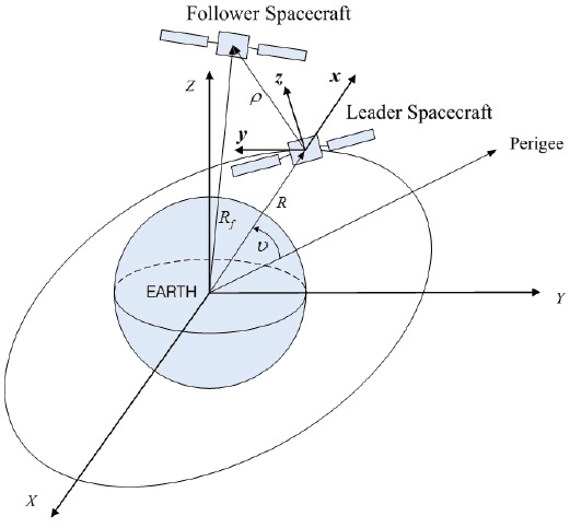
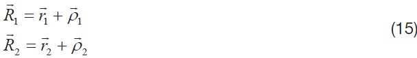
The inertial coordinate system and a rotating local coordinate system are defined for spacecraft formation flying. As shown in Fig. 1, the inertial coordinate system {
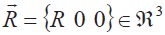
denotes the position vector of the leader spacecraft and
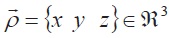
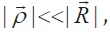
is the relative position vector of the follower spacecraft with respect to the leader spacecraft in the LVLH frame. Then, the position of each follower spacecraft within a formation is given by

The nonlinear equation of the relative motion for elliptic reference orbits can be represented as

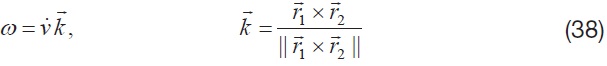
where

is the angular velocity, and
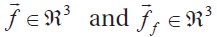
are external forces acting on the leader and follower spacecraft, respectively. When the external forces only act on a central gravitational field, the nonlinear relative dynamics for elliptic reference orbits can be represented as follows:
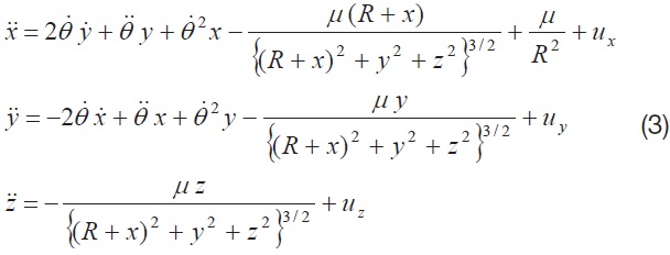
where

is the orbital angular velocity, and
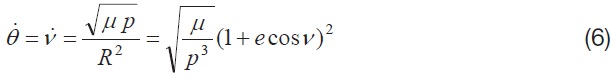
radial, along-track, and cross-track direction, respectively. In orbital mechanics, the radius and angular velocity of the leader spacecraft are given as [16]

where
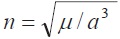
is the natural frequency of the reference orbit.
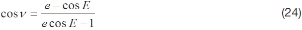
Equation (3) can be expressed using the true anomaly
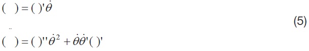
where ( )' and ( )'' denote the first and second derivatives with respect to
the relative motion equation can be expressed as follows:
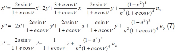
Using Eq. (7), the maneuver problem for the formation reconfiguration is solved and the initial and final conditions are selected in the true anomaly domain to meet the periodicity condition as presented in Ref. [17].
3. Formation Reconfiguration using Impul sive Control Input
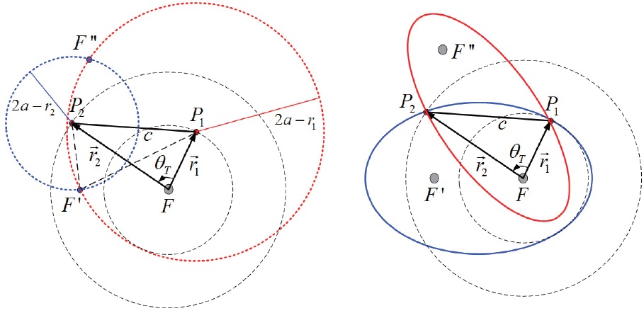
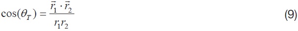
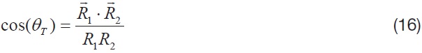
Lambert’s theorem states that the flight time from one point to another depends on the semi-major axis of transfer orbit, the distance of the initial and final points of the arc from the center of force, and the length of the chord joining the points. The chord length,

, as shown in Fig. 2, is defined by the cosine law as follows:

In Fig. 2,
are the position vectors at the initial time
The direction of flight can be defined by the transfer angle; the spacecraft moves along the short way when
To determine the transfer orbit between two position vectors, two foci and semi-major axis should be found. From the definition of the ellipse, the location of the vacant focus and semi-major axis of the transfer orbit can be determined. As shown in Fig. 2, two circles can be drawn having 2
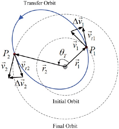
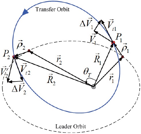
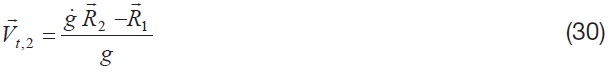
When the transfer orbit is determined, the velocity vectors of the transfer orbot at the initial and final time,
, as shown in Fig. 3, can be calculation by Kepler's equation. Consequently, the velocity changes Δ


where
are velocity vectors of the spacecraft around a planet at the initial and final time. Figure 3 shows the velocity changes using two impulse inputs. The total velocity change can defined as follows:

3.2 Modified Lambert’s Problem for Follower Spacecraft
The transfer orbit for the follower spacecraft connecting two relative position vectors can be solved modifying Lambert’s problem, when the orbital elements of the leader spacecraft and the flight time are known. The geometry of the transfer orbit for the follower spacecraft is illustrated in Fig. 4.
The relative position vectors of the follower spacecraft with respect to the leader spacecraft,
ath the initial time


The position vectors of the follower spacecraft with respect to the Earth at
where
are the position vectors of the leader spacecraft in the ECI frame at
Let us define the velocity vectors of the follower spacecraft at
, respectively. Given two position vectors,
the transfer orbit for the follower spacecraft can be determined through Lambert’s problem as explained in the previous section. The transfer angle can be defined by
The chord length is determined as

Using
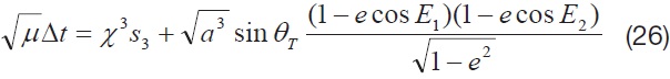
as shown in Fig. 4. The transfer time for the elliptic orbit is defined from Kepler’s equation as follows [7,8]:
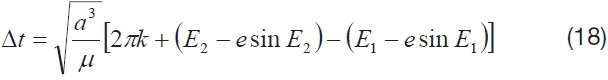
where Δ

where Δ

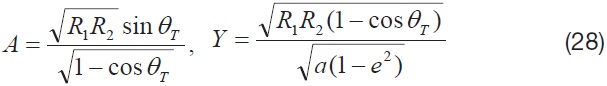
In addition, parameters
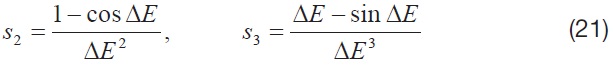
Using Eqs. (20) and (21), Eq. (19) can be expressed as

With trigonometric identity, sin(

The relation between eccentric anomaly
After some manipulation with Eq. (24), Eq. (23) can be expressed as follows:

With the trigonometric identity, Eq. (25) is presented as
The radius is defined as

where
The resulting
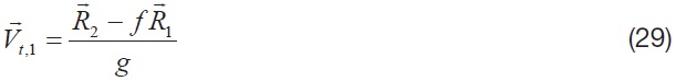
where
Finally, the velocity changes Δ


Consequently, the total velocity change can be calculated as

Note that
are velocities with respect to the Earth and expressed in the ECI frame. Thus, the relative velocity vectors of the follower spacecraft with respect to the leader spacecraft can be expressed as follows:


where
are velocity vectors of the leader spacecraft at
Finally, the relative velocity vectors in the LVLH frame and the orbital elements of the transfer orbit can be found.
4. Numerical Simulation and Analysis
In this section, numerical simulations are performed for the maneuver problem of formation reconfiguration. Using impulsive control input, two maneuvering cases are considered to verify the formation reconfiguration in relative motion: change of the formation radius,
4.1 Radial/Along-Track Plane Formation
In this section, the maneuver for formation reconfiguration in the RAPF is performed using impulsive control input. The orbital elements of the leader spacecraft are summarized in Table 1. To change the formation radius in the RAPF, we consider a situation that the follower spacecraft moves from the initial formation radius of 5,000 m to the final formation radius of 10,000 m. The initial and final conditions are selected to satisfy the periodicity and zero offset condition according to the formation geometry as presented in Ref. [17]. The initial and final conditions of the follower spacecraft in the LVLH frame are summarized in Table 2. The flight time is obtained as 5166.4 seconds given the initial and final conditions as described in Table 2.
[Table 1.] Orbital elements of leader spacecraft
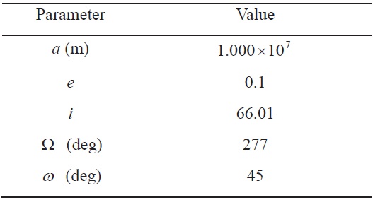
Orbital elements of leader spacecraft
[Table 2.] Initial and final condition (RAPF)
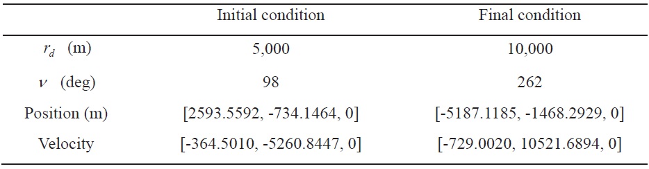
Initial and final condition (RAPF)
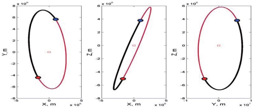
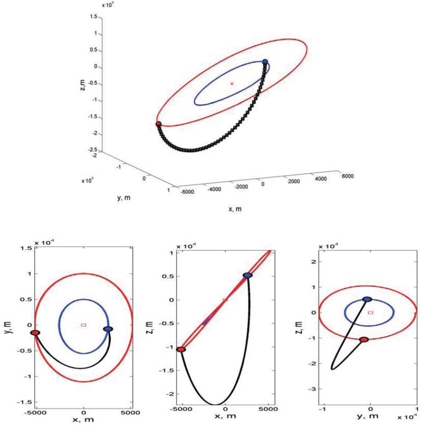
Figures 5?7 show the simulation results for maneuvering in the RAPF. Figure 5 shows the trajectories of the leader and follower spacecraft in the ECI frame; the normal line denotes the trajectory of the leader spacecraft and the thick line transfer trajectory of the follower spacecraft. As shown in Fig. 5, it is difficult to understand the relative motion of the follower spacecraft with respect to the leader spacecraft in the ECI frame. Instead, Fig. 6 transfer trajectory of the follower spacecraft in the LVLH frame. As shown in Fig. 6, the follower spacecraft moves from the initial position to the final position on the
4.2 Along-Track/Cross-Track Plane Formation
In this section, the maneuver for formation reconfiguration in the ACPF is performed using impulsive control input. The orbital elements of the leader spacecraft are same as previous section. To change the formation radius in the ACPF, we consider a situation in which the follower spacecraft moves
[Table 3.] Solution of modified Lambert’s problem (RAPF)

Solution of modified Lambert’s problem (RAPF)
[Table 4.] Initial and final condition (ACPF)
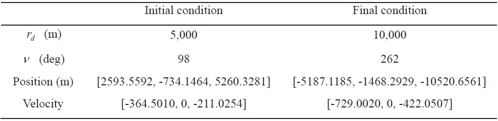
Initial and final condition (ACPF)
from the initial formation radius of 5,000 m to the final formation radius of 10,000 m. The initial and final conditions of the follower spacecraft in the LVLH frame are given by
[Table 5.] Solution of modified Lambert’s problem (ACPF)
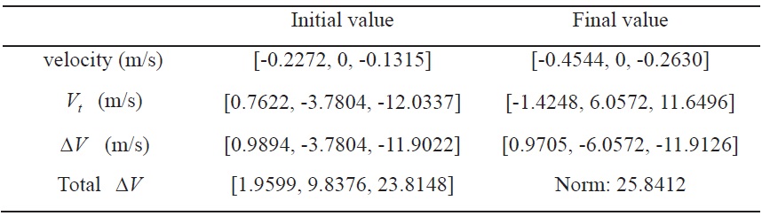
Solution of modified Lambert’s problem (ACPF)
formation geometry in Table 4 as presented in Ref. [17].
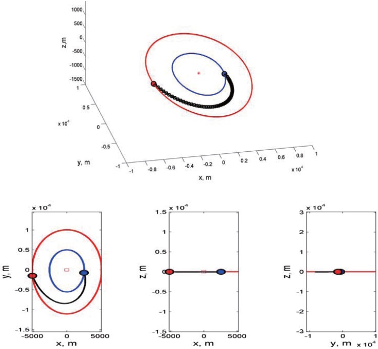
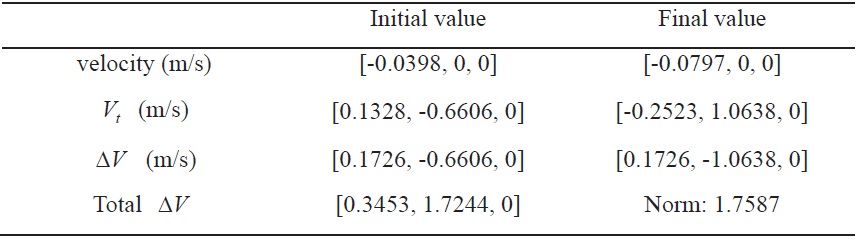
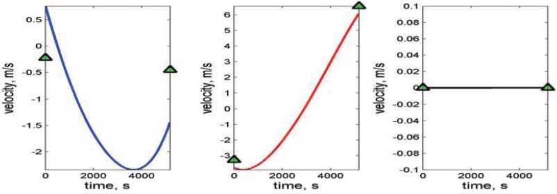
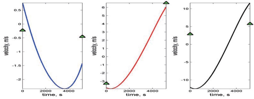
Figures 8?9 show the simulation results for formation reconfiguration using impulsive control input in the ACPF. Figure 8 shows the transfer trajectory of the follower spacecraft with respect to the leader spacecraft in the LVLH frame. Figure 9 shows the velocity history of the follower spacecraft during the maneuver. In Fig. 9, the triangle denotes specified velocities at the initial and final time in the LVLH frame given in Table 4. Therefore, the required velocity change can be obtained by computing the difference between the resulting velocity from the modified Lambert’s problem and the specified velocity. Table 5 summarizes the velocities of the follower spacecraft and △
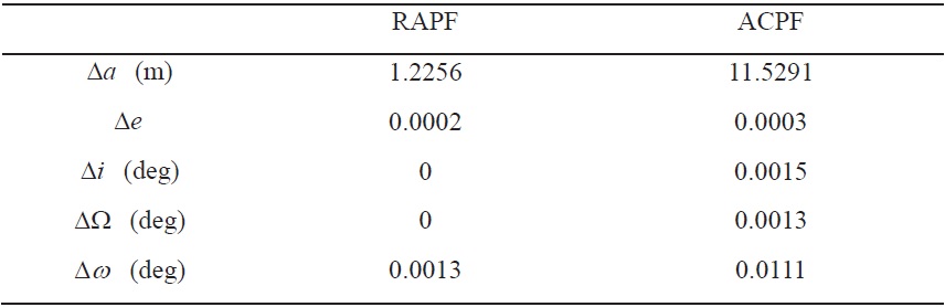
In this section, the simulation results for the formation reconfiguration using impulsive control input in the RAPF and ACPF are analyzed. The simulation results are investigated in terms of the difference of the orbital elements between the transfer orbit and reference orbit with respect to the formation geometry.
As described in Sections 4.1 and 4.2, the transfer orbits are generated where the initial and final positions are arbitrarily chosen in the RAPF and ACPF. By comparing with the orbital elements of the leader spacecraft in Table 1, it is seen that the transfer orbits of two formation reconfigurations have almost same orbital elements, as described in Fig. 5; however, some orbital elements are different. Table 6 summarizes the differences of the orbital elements: (i) between the reference orbit and the transfer orbit in the RAPF as described in Sections 4.1, and (ii) between the reference orbit and the transfer orbit in the ACPF in Section 4.2. These results show the maneuver characteristics of relative motion in the RAPF and ACPF. As shown in Table 6, the difference of the semi-major axis for the ACPF case is much larger than that for the RAPF case. This difference leads to the total velocity change △
[Table 6.] Difference of orbital elements

Difference of orbital elements
between two orbits in RAPF produces a difference in orbital elements including the semi-major axis
A formation reconfiguration using impulsive control input is developed for spacecraft formation flying. To transfer between two position vectors at initial and final time, two impulsive control inputs are generated through modification of the classical Lambert’s problem. The modified method provides the transfer orbit in relative motion for spacecraft formation flying, and therefore the follower spacecraft can change the formation radius and/or geometry with respect to the leader spacecraft. Numerical simulations are performed to solve the maneuver problem for formation reconfiguration in the RAPF and ACPF. These results show the maneuver characteristics of the transfer orbit with respect to the formation type. Through these result, it can be concluded that the transfer orbit for resizing formation radius in the RAPF is related to the coplanar maneuver, and transfer orbit in the ACPF belongs to the combined maneuver of coplanar and non-coplanar maneuvers.