Recently, researches on Micro Aerial Vehicles (MAVs) have been vigorously performed for calamity observation, spraying agricultural chemicals, and military purposes, such as reconnaissance, monitoring, and communication. Moreover, the technology of the MAVs is getting faster, according to the rapid progress of electronic and computer technology. MAV are classified into two categories, fixed and rotary wing types. The rotary wing type MAVs are more advantageous than the fixed wing type ones, as regards VTOL (Vertical Take-off and Landing), omni-directional flying, and hovering performance. Rotary wing type MAVs are classified into quad-rotor type (QRT), co-axial helicopter, and helicopter etc. QRT MAVs have the simplest mechanical structure among them, and the quadrotor we consider to be an underactuated system, with six outputs and four inputs, where the states are highly coupled. To deal with this problem, many modeling approaches have been presented [1,2], and various control methods proposed [3-7]. Bouabdallah et al. presented PID vs. LQ control techniques applied to an indoor MicroQuadrotor [3]. Tayebi et al. studied attitude stablilization of a VIOL quadrotor aircraft [4]. Another PD control method was proposed by Erginer et al. [5]. Feedback Linearization vs. Adaptive Sliding Mode Control for a Quadrotor Helicopter was implemented by Lee et al. [6]. A new robust adaptive-fuzzy control method applied to quadrotor helicopter stabilization was proposed by Coza et al. [7].
Of course, the whole purpose of the MAV is to carry a payload. For the moment, the primary mission assigned to MAVs is aerial observation and surveillance. MAVs are obviously an advantageous solution for missions where a live crew offers no real benefits, or where the risks are too high. In general, for MAVs to carry out the missions under consideration, all aspects of the system will have to be improved: the vehicle itself, payloads, and in particular, sensors, transmission systems, and onboard intelligence.
In this paper, we introduce a configuration of a multi rotor helicopter composed of eight rotors, which is used to solve the problem of the low coefficient proportion between lift and gravity of the Quadrotor MAV. The main characteristics of the configurations are increased payload capacity, quietness efficiency, stability in the wind, and damage tolerance.
A dynamic model is presented. To validate the model, we introduce an intelligent control strategy, and apply it in realtime experiences. The control strategy is based on a Neuro- Fuzzy adaptive controller. Neuro-Fuzzy has been used in a lot of successful applications [8-13]. For example, Spooner et al. [8] and Ordonez et al. [9] proposed a combination of fuzzy systems and neural networks to make adaptive control systems. Melin et al. used a neuro?fuzzy?fractal approach to adaptive control of a model-based non-linear dynamic plant [10]. Lou et al. used a neuro-fuzzy method for modeling and adaptive control of the mechanism [11]. Melin et al. used a neuro?fuzzy?genetic approach to the control of complex electrochemical systems [12]. Er et al. designed a dynamic fuzzy neural networks controller for a Selective Compliance Assembly Robot Armand (SCARA) with realtime implementation [13]. But these are based on type-I fuzzy sets. With the higher control accuracy requirements, the type-II fuzzy neural network [14-17] that has been developed recently, has better performances than the type-I fuzzy neural network. For example, system identification by using a type-II fuzzy neural network was developed by Lee et al. [14], and Wang studied dynamic optimal training for interval type-II fuzzy neural networks [15]. A double axis motion control system and dynamic time-varying system identification with type-II fuzzy neural networks was designed by Chen et al. [16-17]. This paper is to apply type- II fuzzy neural networks to control the attitude of the Eight- Rotor MAV.
More recently, there are many papers discussing how to improve the stability of fuzzy-neural controllers. It is well known that sliding mode control provides a robust means for controlling a nonlinear dynamic system with uncertainties. Lin [18] proposed an interval type- II fuzzy-neural network direct adaptive sliding mode control for SISO nonlinear systems. In this paper, we develop a gain adaptive sliding mode controller based on an interval type-II fuzzy neural network [18-20] identification and Lyapunov synthesis approach for the Eight-Rotor MAV, which is a MIMO nonlinear system. By introducing an interval type-II fuzzy neural network to approximate the unknown nonlinear functions of the dynamic systems, through tuning by the desired adaptive law, we introduce the Lyapunov synthesis technique in this paper. Furthermore, by incorporating the Lyapunov design approach and sliding mode control method into the adaptive fuzzy-neural control scheme to derive the control law, the advocated design methodology not only assures closed-loop stability, but also a desired tracking performance can be achieved for the overall system, based on a much relaxed assumption.
This paper is organized as follows: the attitude dynamic model of the Eight-Rotor MAV is given in Section 2. A brief illustration of an interval type-II fuzzy neural network is presented in Section 3. A gain adaptive sliding mode controller based on interval type-II fuzzy neural network identification is constructed in Section 4, which is also devoted to the stability analysis of the control scheme. A platform description and some experiences are given in Section 5, and Section 6 contains concluding remarks.
2. Dynamic modelling of the Eight-Rotor MAV
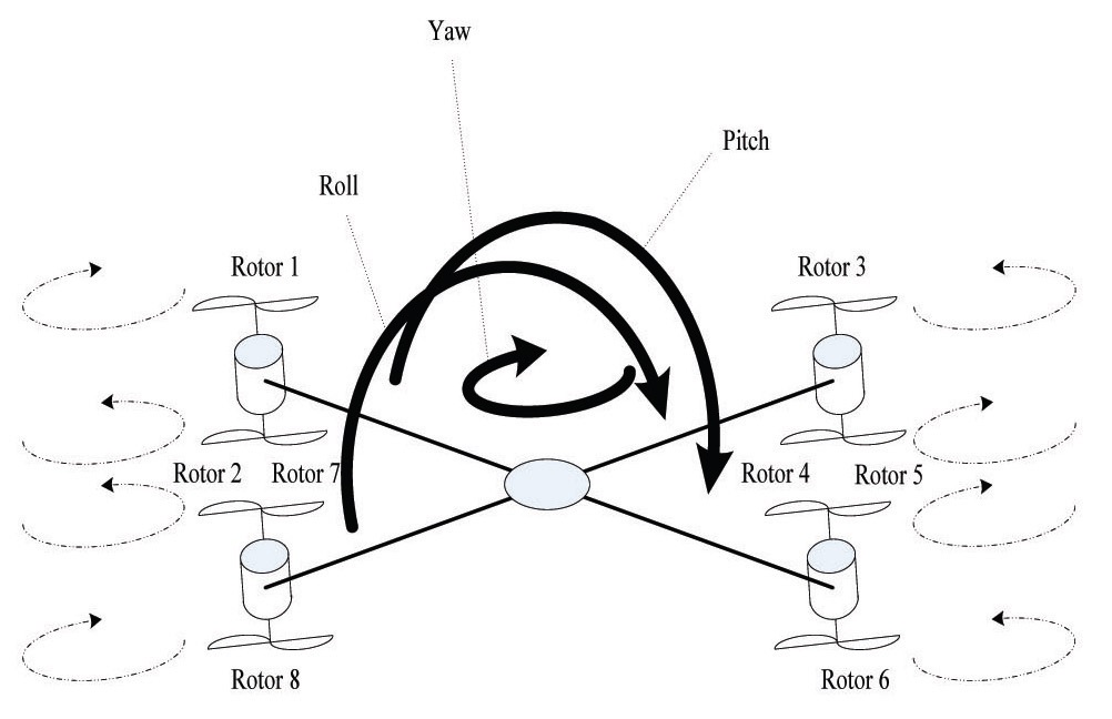
The EightRotor is very well modeled, with eight rotors in a cross configuration. This cross structure is quite thin and light; however, it shows robustness, by mechanically linking the motors. Each propeller is connected to the motor through reduction gears. All the propellers axes of rotation are fixed and parallel. These considerations point out that the structure is quite rigid, and the only things that can vary are the propeller speeds. Neither the motors nor the reduction gears are fundamental, because the movements are directly related just to the propellers velocities, as can be seen in Fig. 1.
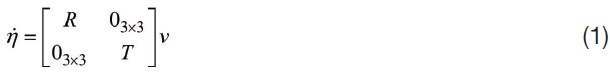
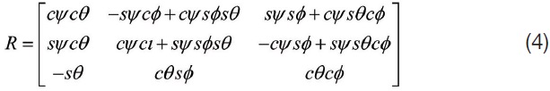
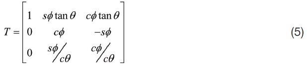
The first step before control development is an adequate dynamic system modeling. Let us consider two frames that have to be defined: the earth inertial frame (E-frame) [10]; and the body-fixed frame (B-frame). Eq. (1) describes the
kinematics of a generic 6 degree of freedom rigid-body:
where, the


The notation O3×3 means a sub-matrix with dimension 3 times 3 filled with all zeros, while the rotation
The dynamics of a generic 6 degree of freedom rigid-body take into account the mass of the body m and its inertia matrix I, which is calculated in this work. The dynamics are described by Eq.(6)
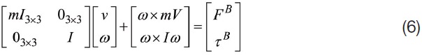
where, the notation I3×3 means a 3 times 3 identity matrix.

Hence the last vector contains specific information about its dynamics. Γ can be divided into three components, according to the nature of the Eight-Rotor contributions.
The first contribution is the gravitational vector
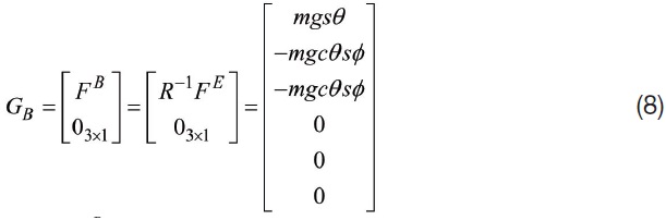
where
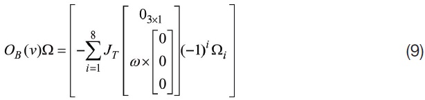
The second contribution takes into account the gyroscopic effects produced by the propeller rotation, since four of them are rotating clockwise, and the other four counter clockwise. The overall rotor speeds are, in general, not equal to zero. In imbalance, when the algebraic sum of the addition, roll or pitch rates are also different from zero, the Eight-Rotor experiences a gyroscopic torque, according to Eq. (9). OB(v) is the gyroscopic propeller matrix, and
The third contribution takes into account the forces and torques directly produced by the main movement inputs. From aerodynamic consideration, it follows that both forces and torques are proportional to the squared propellers’ speed. Therefore the movement matrix
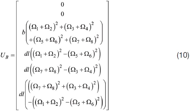
where, l is the distance between the center of the Eight-Rotor and the center of a propeller, b means the square of the motor speed-lift scaling factor, d means the force-moment scaling factor, and U1, U2, U3 and U4 are the movement vector components. Their relation with the propeller speeds comes from aerodynamic calculus. Therefore, all the movements have a similar expression, and are easier to control. It is possible to describe the Eight-Rotor dynamics considering these last three contributions, according to Eq. (11).

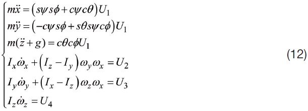
Eq. (12) shows the previous expression not in a matrix form, but in a system of equations:
where, the propellers’ speed inputs are given through Eq.(13)
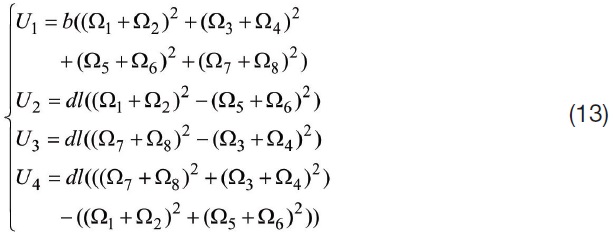
The dynamics of the Eight-Rotor are well described in the previous section. However the most important concepts can be summarized in Eqs. (12) and (13). The first one shows how the Eight-Rotor accelerates, according to the basic movement commands given. The second equation explains how the basic movements are related to the propellers’ squared speed. The goal of the Eight-Rotor stabilization is to find those values of the motors’ voltage that maintain the helicopter in a certain position required in the task. This process is also known as inverse kinematics and inverse dynamics. Unlike the direct ones, the inverse operations are not always possible, and are not always unique. For these reasons, their consideration is much more complicated.
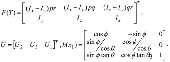
Making the outputs tracks the attitude of the Eight-Rotor MAV, by designing the control torque U. Arranging the above dynamic equations for designing the control scheme conveniently, the attitude control model of the Micro Aircraft Vehicle obtained can be expressed as:
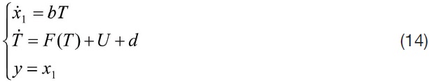
where,
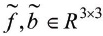
Next, we propose
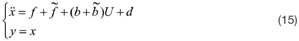
where,
means the uncertainty function vector caused by attitude perturbations, and each component expression of
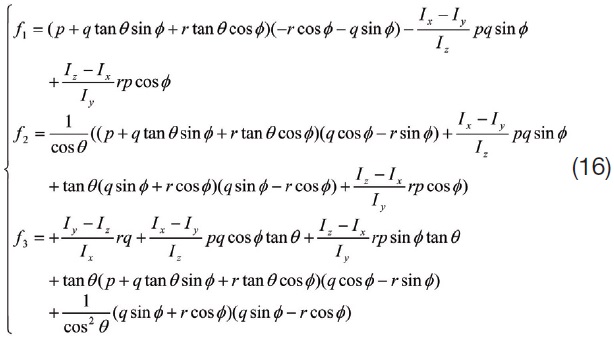
Aerodynamic characteristics parameters will get perturbations, resulting from flying conditions or changes in flying attitude. At the same time, external gusts of wind and flow cannot be ignored. Thus, the control system of the Micro Aircraft Vehicle is a MIMO nonlinear system with uncertainty and perturbations.
3. Introduction of the Interval Type-II Fuzzy Neural Network
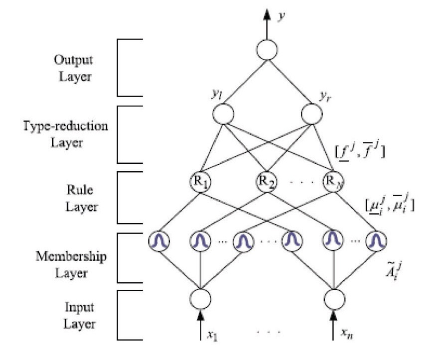
The structure of ITIIFNN [16-17] is depicted in Fig. 2; each rule in ITIIFNN is of the first Takagi-Sugeno-Kang (TSK) type. The detailed mathematical functions of each layer are introduced as follows:
Layer 1 (Input layer): This layer defines the input variables that first enter the ITIIFNN.
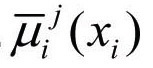
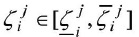
Layer 2 (Membership layer): In this layer, each node performs an interval type-II fuzzy MF. The FOU of this MF can be represented as an interval, bound by lower MF
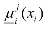
and upper MF
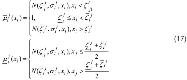
where,
and

Layer 3 (Rule layer): Each node in this layer corresponds to one fuzzy rule, and performs a fuzzy meet operation, to obtain a firing strength
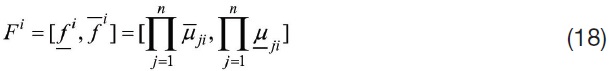
Layer 4 (Type-reduction layer): This layer is used to implement the type-reduction, and the center-of-sets type reduction method is adopted here. The centroid of the type-II fuzzy set that can be represented by [
[Table 1.] Response data of three attitude angles

Response data of three attitude angles
where,
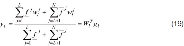
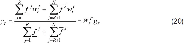
Layer 5 (Output layer): Each output node corresponds to one output variable, and acts as a defuzzifier. Hence, the defuzzified output is shown as:

Remark: Initially, there are no fuzzy rules in ITIIFNN. All of the rules are generated online by the structure learning, which not only helps automate rule generation, but also locates good initial rule positions for subsequent parameter learning. Furthermore, the structure and parameter adjustment are performed simultaneously.
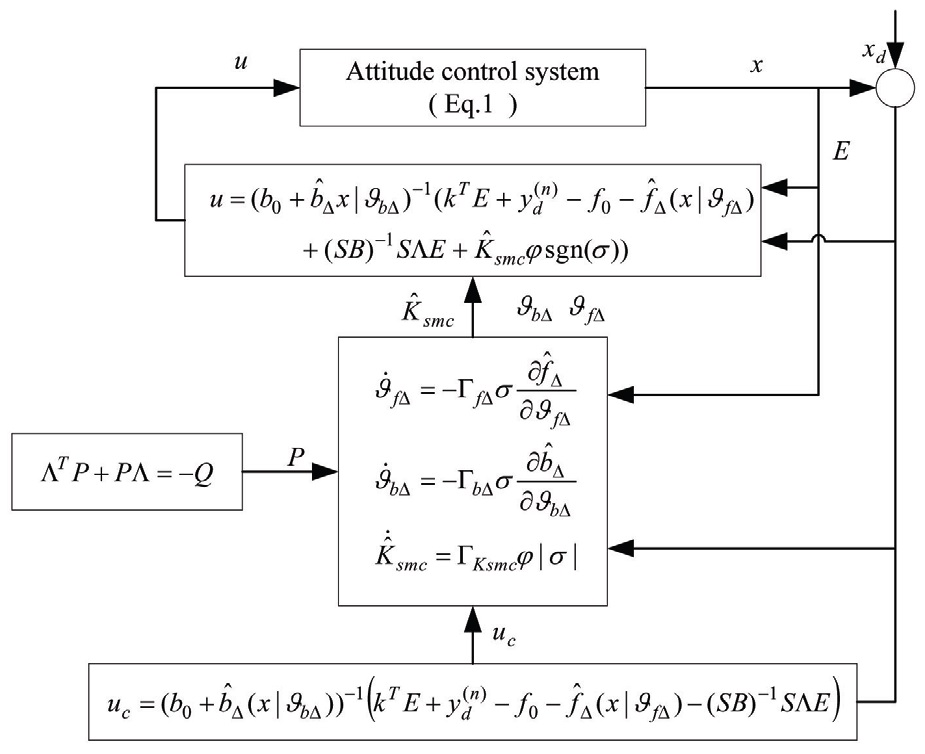
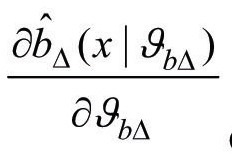
To begin with, our objective is to use the ITIIFNN, as shown in Fig. 3, to approximate the uncertainty function f and nonlinear function b, for the adaptive sliding model controller on-line. Then, we analyze the stability of the proposed adaptive sliding model controller based on ITIIFNN through the Lyapunov stability theorem, in the meantime tuning the parameters of the interval type-II fuzzy neural network and gain of the sliding mode control on-line, by adaptive laws based on the Lyapunov synthesis approach.
Proposing

then, the error dynamic equation with uncertainty and external disturbances can be expressed as:

where,
In the meantime, the selection of
Taking

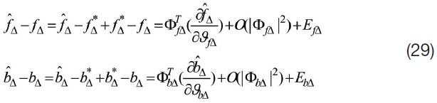
Proposing that
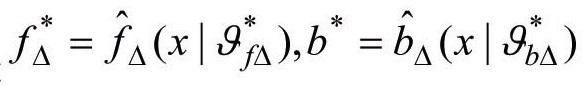
with respect to the optimal estimations of
the minimum estimation
error is defined as:

where,
Gaussian membership function standard deviation
in the Taylor series expression near
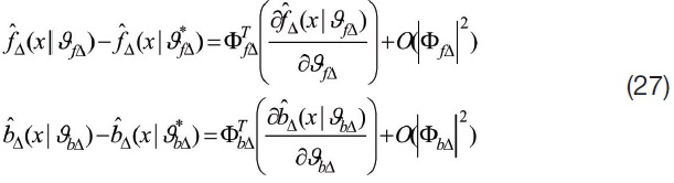
where,

are representative of the higher-order item. Each item of
is expressed as:
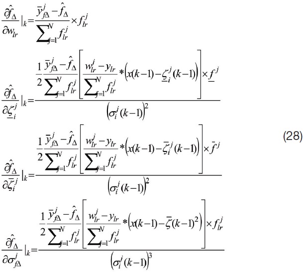
Replacing the
can be achieved. Hence, we obtain:
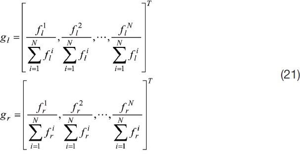
Then,
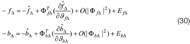
By using Eq. (21), Eq. (14) can be rewritten as:
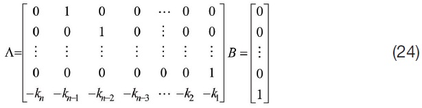
Define

Then, the error dynamic Eq. (22) could be simplified as:
Owing to the given ?,

where, ? is a stable matrix. In view of the value principle of K, there exists positive symmetric matrices Q, which guarantees the unique positive symmetric solution P of the Lyapunov equation.

Defining the switching surface as:

where,

Then the equivalent control variable

when

when

In this time, Eq. (40) turns to be:
Taking
as the disturbances, and substituting them into the disturbance item d in Eq. (40), the expression is shown as:
Then,
Now, Eq. (34) can be expressed as:

Next, make the following assumptions:
If the above assumptions hold true, the following equation can be obtained as:

where,
For enhancing the system robustness with the existences both
where,
is the estimated value of
, and also meeting the condition that
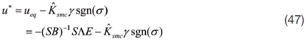
. Finally, the actual control variable
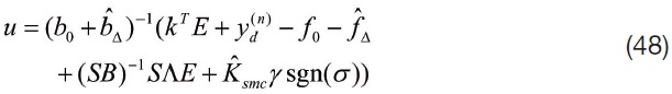
The whole gain adaptive sliding mode controller (GASMC) based on an interval type-II fuzzy neural network (ITIIFNN) identification algorithm has been given in Fig. 2.
Theorem 1. Consider the error dynamic system Eq. (23), if the control variable
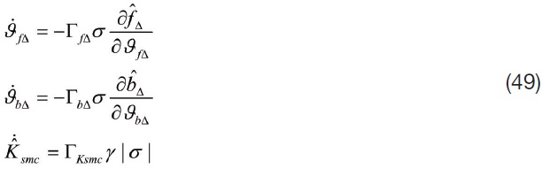
where, Γ
Proof . Define a Lyapunov function as:
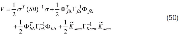
Then, the time derivative of the Lyapunov function V becomes:
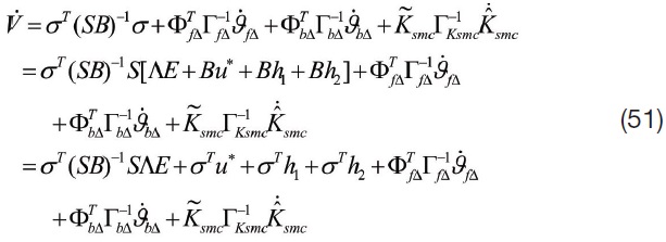
Using Eq. (44), Eq. (48) and Eq. (50), the time derivative of V can be derived as:

And considering the inequality of Eq. (38), then the time derivative of V can be obtained as:
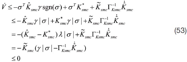
This is to say that

according to the Lyapunov stability theorem, because the switching surface is stable, then

In other words, the error dynamic system Eq. (23) is uniform asymptotic stable.
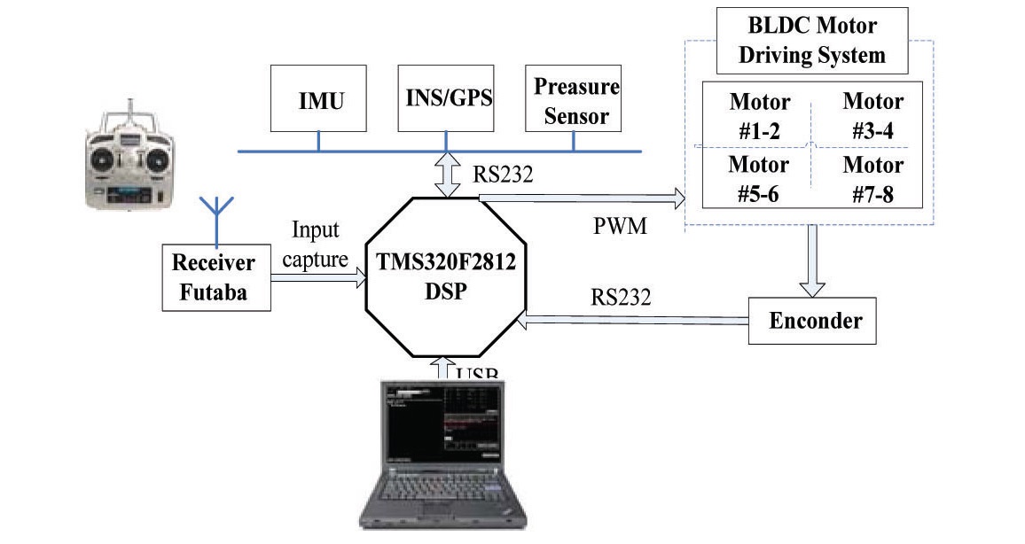
A schematic view of the aerial control platform using TMS320F2812 is shown in Fig. 4. The Eight-Rotor MAV has four blades, driven by eight BLDC motors, mounted at each end of the body frame. The Encoders were used for measuring the speed of each motor. The INS data are updated at 5 Hz, and the static pressure sensor measures are provided at a rate of 50 Hz. The low-cost IMU outputs raw data from 3 accelerometers, 3 gyro meters and 3 magnetometers to the flight control computer, which receives all these sensor data through an RS-232 serial port. The on-board flight control computer is TMS320F2812 (DSP), which runs at 29.4M Hz, with 512k flash memory, including eight serial ports, eight channels with programmable gains, 24-bit analog input, six programmable Pulse Width Modulation (PWM) outputs, and supports floating point calculations.
To avoid signal interference between sensor signals and the motors PWM, two independent power supplies are supplied. One battery is used to feed the eight electric motors, which are controlled using PWM, the other battery is used to feed the microcontroller and the sensors, and by adequate grounding, the interference is largely reduced.
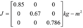
The Eight-Rotor Micro Aircraft Vehicle is characterized by a nominal main body inertia matrix :
The fuzzy rules in the ITIIFNN can be generated automatically, by using the on-line adaptive laws to obtain suitable-structure neural networks, so the weighting factor is set to be zero
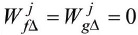
initially. The other parameters can be chosen as:
The parameters of the sliding mode used here are chosen as:
Ksmc(0) = [1.2×105,104]T,
Γsmc = diag(4.5×104,4.5×104).
The initial attitude angle is set to be zero
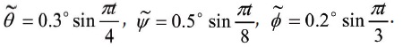
Considering the torque perturbations caused by the Micro Aircraft Vehicle body and Micro Aircraft Vehicle wing, the uncertainty functions are set to be [0.2° cos
For the purpose of comparison, several different kinds of control scheme are conducted, to demonstrate the effectiveness of the proposed approach. We will apply the conventional adaptive sliding mode controller [21], a type-I fuzzy neural network based sliding mode controller [22-23] and an interval type-II fuzzy neural network identification based gain adaptive sliding mode controller, to let the Micro
Aircraft Vehicle system track the reference attitude trajectory.
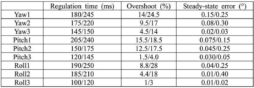
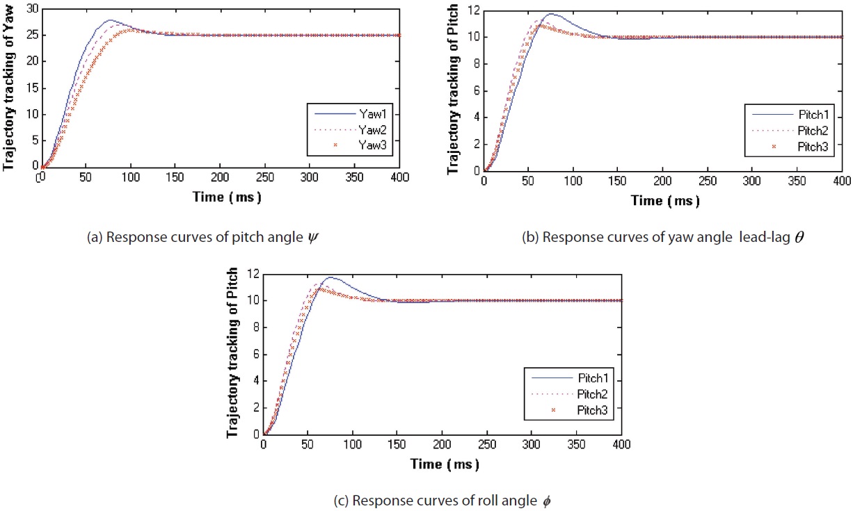
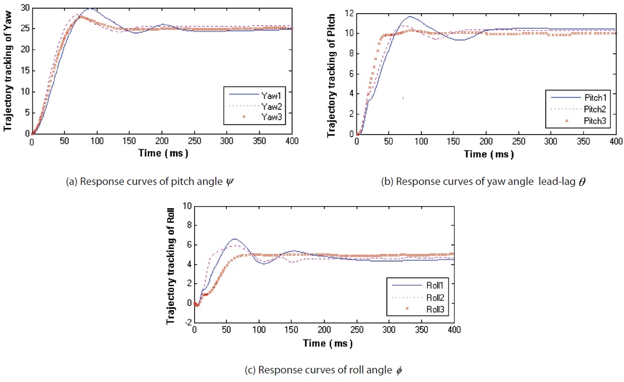
The yaw Angle, pitch Angle and roll Angle, three attitude angles of trajectory tracking simulations, have been made as follows: Fig. 5 shows the trajectory tracking response curve of the three angles, under the circumstance without external disturbance and uncertainty. Fig. 6 shows the trajectory tracking response curve of the three angles, under the circumstance with external disturbance and uncertainty. Subscript Numbers under attitude Angles correspond to three kinds of controller: “1” is representative of the conventional adaptive sliding mode controller; “2” is representative of the type-I fuzzy neural network based sliding mode controller; and “3” is representative of the type-II fuzzy neural network identification based adaptive sliding mode controller.
The above two experimental results indicate that tracking performances can be guaranteed under the three different control schemes. The conventional adaptive sliding mode control scheme responds fast, but its overshoot is somewhat large; the Type-I fuzzy neural network based sliding mode control scheme has smaller steady-state error, but with longer regulation time; the Type-II fuzzy neural network identification based gain adaptive sliding mode control has better control accuracy, and smaller overshoot. The control accuracy decreases under uncertainty factors and external disturbances for all of the three control schemes, but could satisfy the performance standard of the control system; furthermore, the Type-II fuzzy neural network identification based gain adaptive sliding mode control scheme gives better performances, compared with the other ones.
Arranging the above simulation results from Fig. 5-Fig. 6, then the response data of the three attitude angles are listed in Table 1. From Fig. 5-Fig. 6 and Table 1, we can see that not only from the nominal system, but also from the system with uncertainty and external disturbances in Fig. 6, it can be seen that the conventional adaptive sliding mode control scheme produces greater overshoot and steady-state error; the Type-I fuzzy neural network based sliding mode control scheme produces large overshoot and small steady-state error; and the Type-II fuzzy neural network identification based gain adaptive sliding mode control scheme produces smaller overshoot and small steady-state error.
In this paper, we have presented the dynamical modeling and intelligent control strategy of a MAV having eight rotors. One of the main characteristics of these configurations is the damage tolerance and increased stability in the wind. A novel adaptive sliding mode controller based on an interval type-II fuzzy neural network is developed, to handle uncertainties caused by both rule uncertainties and attitude angle perturbations, for an attitude angle control system involving external disturbances. The Lyapunov stability theorem has been used to test the asymptotic stability of the closed-loop system. Therefore, the parameters of the interval type-II fuzzy neural network and gain of the sliding mode control can be tuned on-line, by adaptive laws based on the Lyapunov
synthesis approach. From the experimental and comparison results, it is obvious that the tracking performance obtained from the proposed methodology is better than the type-I fuzzy neural network sliding mode controller and conventional adaptive sliding mode controller, not only in the nominal system, but also in the system with uncertainty factors and external disturbances. Thus, the experimental results have demonstrated the effectiveness of the proposed algorithm.