This paper presents a control effectiveness analysis of the hawkmoth Manduca sexta. A multibody dynamic model of the insect that considers the time-varying inertia of two flapping wings is established, based on measurement data from the real hawkmoth. A six-degree-of-freedom (6-DOF) multibody flight dynamics simulation environment is used to analyze the effectiveness of the control variables defined in a wing kinematics function. The aerodynamics from complex wing flapping motions is estimated by a blade element approach, including translational and rotational force coefficients derived from relevant experimental studies. Control characteristics of flight dynamics with respect to the changes of three angular degrees of freedom (stroke positional, feathering, and deviation angle) of the wing kinematics are investigated. Results show that the symmetric (asymmetric) wing kinematics change of each wing only affects the longitudinal (lateral) flight forces and moments, which implies that the longitudinal and lateral flight controls are decoupled. However, there are coupling effects within each plane of motion. In the longitudinal plane, pitch and forward/backward motion controls are coupled; in the lateral plane, roll and side-translation motion controls are coupled.
Insects perform highly maneuverable yet stable flight that is rarely found from manmade fixed- or rotary-wing aircraft. It is also remarkable that they manage all these maneuvers through only a pair of wings, whereas manmade aircraft utilize thrusters and various other control surfaces, such as flaps, rudders, and ailerons, to maintain their flight. The wings of the insect can be defined to have three independent rotational degrees of freedom (stroke positional, feathering, and deviation angle) [1], and it is believed that the insect can control each of them, with their complex muscles and exoskeleton structure. However, when it comes to an engineered implementation in an insect-inspired micro air vehicle (MAV), there are extreme difficulties, because of the very tight weight budget of the system. At present, only a limited number of actuators and limited complexity of mechanisms are possible to be installed in a flyable flapping wing micro air vehicle (MAV) [2], thus the control characteristics of the system can easily be underactuated. Therefore, the key thing for implementing flight control to the flapping MAV is how to obtain full control authorities to all of the six degrees of freedom motions, with a limited number of possible control inputs.
To better understand the fundamental mechanics of the flight control of the insect, and to utilize the knowledge for realizing manmade flapping MAVs, several interdisciplinary studies between biology and aerospace engineering have been conducted. High-speed footage recording/processing techniques for the stimulated (disturbed) flying insect [3,4] are used to investigate bio-inspired control strategies of the insects: which sensory organ it uses, which state it feeds back, which muscle it activates, and consequently, which control strategy it uses to evade flight instability. However, this inference process has a limitation, in that it can only provide us with input/output sets and inferred control strategy based on hypothesis testing. A simplified mathematical modeling of the insect flight dynamics and hardware development/test has also been conducted [5-8]. Through this mathematical modeling approach, more direct clues can be provided, such as a quantitative relation between given control inputs, and the consequent dynamic responses. However, several assumptions for a simplified modeling make it hard to capture the time-varying nonlinear characteristics of the insect flight dynamics. Frequently used assumptions are cycle-averaged aerodynamics, simple single rigid body equations of motion that ignore the inertia effects of flapping wings, and linearization of the equations of motion.
In this study, an at-scale multibody dynamic model of the hawkmoth
[Table 1.] Wing morphological data

Wing morphological data
[Table 2.] Body morphological data

Body morphological data
the author’s previous studies [10,11]. Changes in six degrees of freedom forces and moments with respect to the variation of the three angular degrees of freedom wing kinematics are investigated, and their characteristics are analyzed.
2.1 Insect model and coordinate systems
The hawkmoth
All three body components (head, thorax, and abdomen) and two wings are independently modeled, for a multibody dynamic model of the hawkmoth (Fig. 1 (a)). The head, thorax, and abdomen are connected to each other via a fixed joint, which allows no translation or rotation. The two wings are connected to the thorax via a 3-DOF revolute joint, for the wing kinematics. The body and wing morphological data are referred from measurement data [13,14], and these are tabulated in Tables 1 and 2.
The parameters in Table 1 denote:

is mean chord;
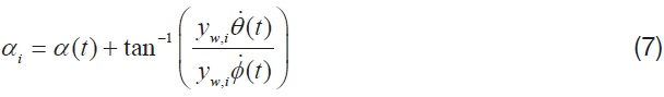
Four coordinate systems are required to describe the dynamics of the hawkmoth model: 1) wing-fixed [
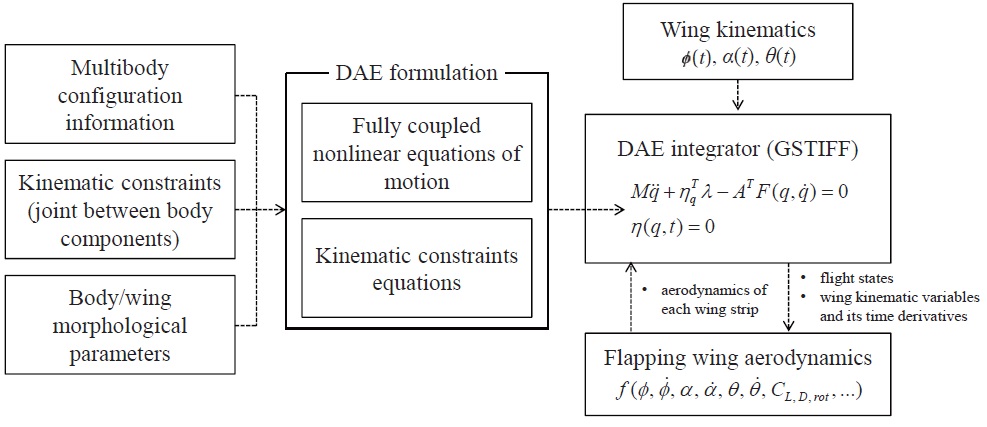
To establish a multibody dynamic model of the hawkmoth, as shown in Fig. 1 (a), we used a multibody dynamics code (
a user-given nultibody configuration (as in Fig. 1 (a)). A generic form of this DAE system is:
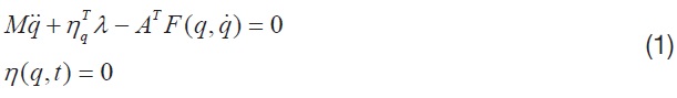
where,
For the forcing terms to the system, here the aerodynamics on the flapping wings are independently coded with
A block diagram, showing the modules used in multibody dynamic modeling and simulation of the hawkmoth, is given in Fig. 3.
2.2 Aerodynamics for the flapping wings
The aerodynamic model used in this study is based on a blade element approach, which is widely used by various research groups [8,15,16]. The blade element approach assumes a wing to be divided into many chord-wise aerodynamic strips. Then the aerodynamics generated from each strip are integrated along the span-wise direction, to calculate the whole wing’s aerodynamic characteristics. Interactions between the wing and wake, or wing and body, are not considered in this aerodynamic model.
In this study, a total of five strips for each wing are used for the application of the blade element approach (
Eqn. 2 shows the components of an instantaneous aerodynamics, developed from a flapping motion of the wing [1].

Among the four major aerodynamic components, the aerodynamics generated from a translational and a rotational motion of the wing is modeled for this study. The translational component is a quasi-steady term, which is a function of the effective angle of attack of the wing strip (
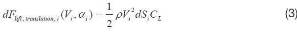


where,
is the mean chord of each aerodynamic strip, and
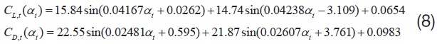

Here, all the areodynamic coefficients (
and the location of the nondimensional axis of rotation
where
2.3 Definition of wing kinematics control input variables
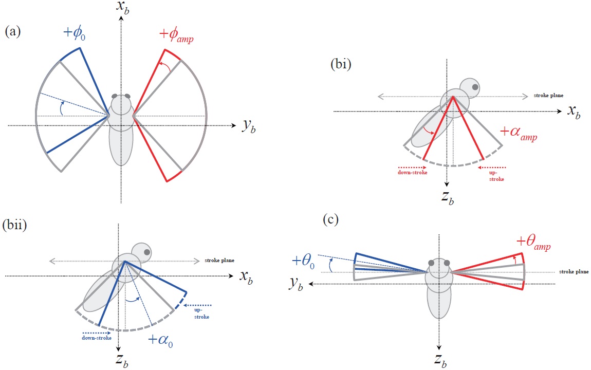
The motion of the insect wing can be defined with three independent angular degrees of freedom at the wing-base pivot: 1)
Based on this wing kinematics definition, the motion of each rotational degree of freedom is defined with a sinusoidal function, to reproduce the periodic wing beat motion of the insect flight. Eqns. 10 to 12 show the wing kinematics function for each rotational degree of freedom:

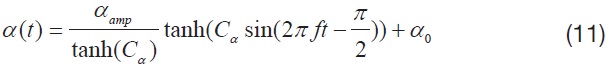


where,
Each kinematics function has two variables, which are the amplitude and bias; and the variation of these two variables is used to evaluate the control effectiveness of the hawkmoth model. All amplitude control variables have nominal values of:
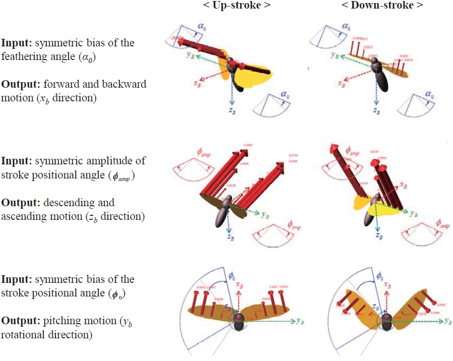
The abovementioned wing kinematics control input variables are depicted in Fig. 4. Each wing has three rotational degrees of freedom, and each rotational degree of freedom has two control variables; hence a total of 12 control input variables are defined, for both left and right wings. However, to obtain more intuitive results, control variable sets are divided into six symmetric and six asymmetric inputs. The
symmetric inputs indicate that the control inputs to the left and right wing are identical, whereas the asymmetric inputs mean that the left and right wing have different control inputs, defined by Δ
The abovementioned control input variable sets for the wing kinematics are given to the hawkmoth model, to investigate their effect on the 6-DOF forces and moments. Overall, the result shows that the symmetric control
[Table 3.] Range and nominal values of each control input variable for the wing kinematics
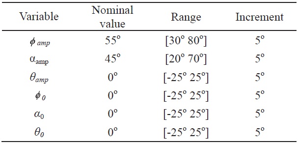
Range and nominal values of each control input variable for the wing kinematics
inputs affect the longitudinal forces and moments, and the asymmetric control inputs affect the lateral forces and moments. Therefore, control inputs for the longitudinal motions and lateral motions are almost decoupled.
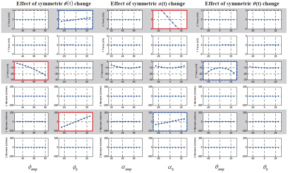
Fig. 5 shows the 6-DOF forces and moments variation with respect to the symmetric wing kinematics control
inputs. The ordinate indicates 6-DOF forces and moments: from above, F
The results show that the symmetric bias of the feathering angle (
motion (
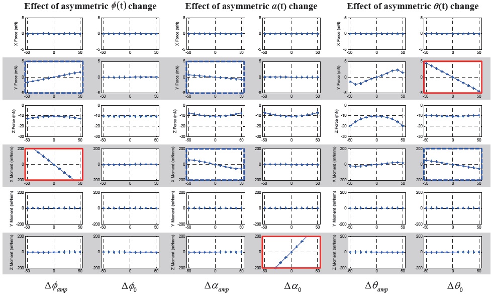
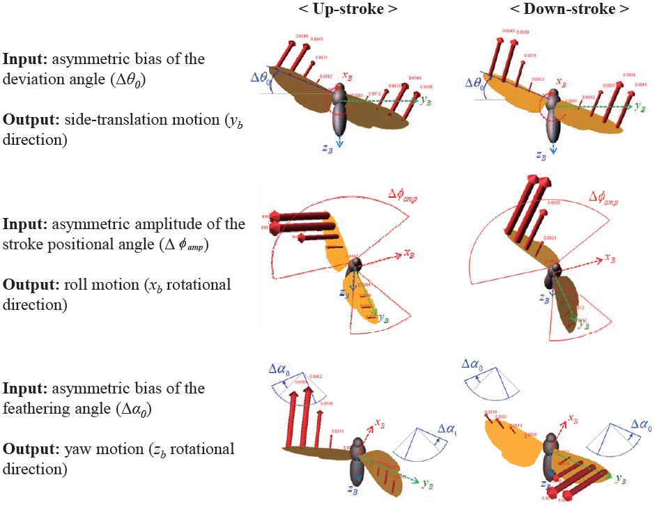
Fig. 7 shows the 6-DOF forces and moments variation with respect to the asymmetric wing kinematics control inputs. The asymmetric control inputs are defined in section 2.3. The ordinate indicates 6-DOF forces and moments: from above,
The results show that the asymmetric bias of the deviation angle (Δ
3.3 Coupling effect of control inputs
As shown in the Figs. 5 and 7, some control input variables affect not only a single directional force or moment (graphs with thick solid border), but they also simultaneously affect two or three forces or moments (graphs with thick dashed border). This means that there is a coupling effect between DOFs with respect to a single control input variable. However, there is not much coupling between longitudinal and lateral DOFs, except only for the longitudinal up/down motion with the lateral dynamics.
In the longitudinal DOFs (
In the lateral DOFs (
In terms of a cross-coupling between motion planes (longitudinal and lateral), there is a longitudinal force component,
A control effectiveness analysis is conducted using a multibody dynamics model of the hawkmoth
For the longitudinal flight: 1) the symmetric bias of the feathering angle (
For the lateral flight: 1) the asymmetric bias of the feathering angle (Δ
From the coupling effect analysis, reduction in the number of necessary control input variables is achieved. Among all twelve possible combinations of control variables for three rotational degrees of freedom of the wing, only four of them (


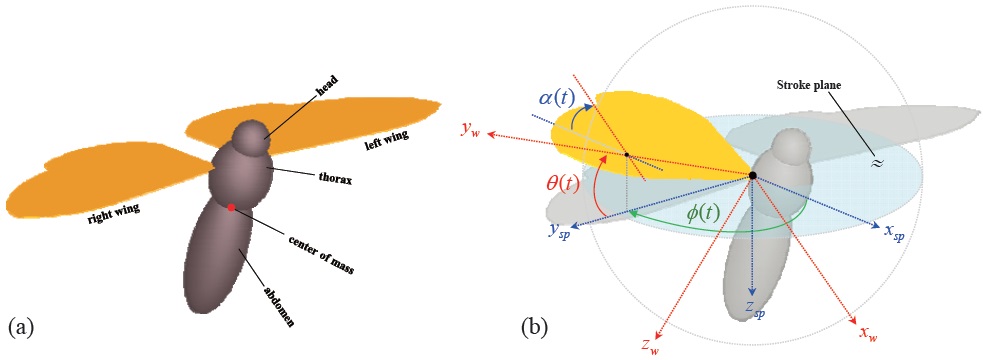
![Definition of the coordinate systems: wing-fixed frame [xw yw zw] is attached to the wing-base pivot, and moves in accordance with the wing motion; stroke-plane frame [xsp ysp zsp] has its origin at the wing-base pivot, and attached to the thorax, and each wing has its own stroke plane; body-fixed frame [xb yb zb] is attached to the center of mass, and defined parallel to the stroke-plane frame.](http://oak.go.kr/repository/journal/12085/HGJHC0_2013_v14n2_152_f002.jpg)