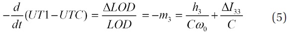
Units of time; ‘hour’, ‘minute’, and ‘second’ were originally defined as the time fractions of one average solar day. Universal time (UT) was originally established by the Earth’s spin rotation. Later, perturbation of length of day (LOD) was recognized, and time units have been redefined by more stable oscillation in cesium atom. UT1 and UTC were defined distinctly as follows; UT1 = ‘time based on the Earth’s spin rotational angle’, and UTC = ‘time kept by atomic clocks at the mean sea level’. To compensate the accumulation of time delay in UT1 due to Earth’s secular deceleration of tidal origin, leap seconds have been applied, so that the difference between UT1 and UTC may not grow bigger than 0.9 second. Seasonal variation of LOD has been clearly recognized since the advent of quartz clock in 1950s. Nowadays, the perturbation in LOD is accurately monitored with sub-microsecond accuracy.
Any position on the Earth’s surface can conveniently be represented by its latitude and longitude, which are two angles defined with respect to the Earth’s reference ellipsoid. Reference Pole (formerly known as the Conventional International Origin), the north pole of the ellipsoid, was determined by the pole position at the beginning of the last century (1900 - 1905). However, the present Earth’s rotational pole is several meters away from the Reference Pole. In fact, true pole position on the Earth varies in complicated way. The relative displacement of the Earth’s pole with respect to the Reference Pole is called polar motion, while polar wander is referred to the long time trend of pole drift. Obviously the exact pole position should be known for the coordinate conversions - from Terrestrial Reference Frame to Celestial Reference Frame and for vice versa. It is noted that precession/nutation should be known together with the polar motion for those conversions. While precession and nutation are being predicted with sub-milliarcsec accuracy for next tens years (Wallace & Capitaine 2006), modeling of polar motion cannot be done at such level due mainly to nonlinear effects in the atmosphere and ocean. Formerly, polar motion was monitored by a consortium, called the International Latitude Service (ILS). Nowadays, the International Earth Rotation and References Service (IERS) supports the information of LOD and polar motion on daily basis. After the advent of space geodetic techniques in 1980s, the measurement accuracy of Earth’s spin rotational perturbation was enhanced greatly (Cerveira et al. 2007). Single space geodetic technique may yield polar motion estimate, however, combined solution is more accurate and stable. It is noted that VLBI is unique discipline to determine UT1. Recently, Ring Laser Gyroscope emerged as a promising tool to measure the instantaneous Earth’s angular velocity (Schreiber et al. 2011 and references therein). Followings are two general references for Earth rotational variations; one - introductory and the other - technical catalog (McCarthy & Seidelmann 2009, Petit & Luzum 2010).
In this study, from the IERS datasets of Earth rotation parameters, different periodic components (from secular to sub-weekly) of LOD and polar motion are extracted by spectral windowing; band-pass in frequency domain and consecutive inverse Fourier transformation. The characteristics of each acquired period band signals are described and examined. Further discussions including the possible causes of certain perturbations of them are given.
2. EARTH’S SPIN ROTATIONAL PERTURBATION THEORY: BRIEF REVIEW
In this section, the equation of motion for the Earth’s spin angular velocity perturbation is stated in the body fixed frame. First, the general equation of motion for rigid body rotation and Euler’s equation for wobble are derived. Further considerations for more realistic Earth are given after then.
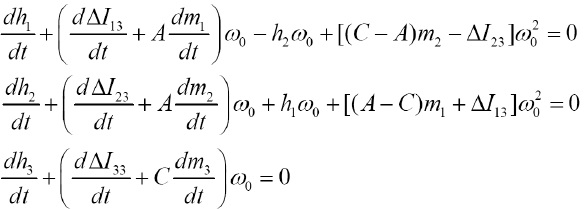
The governing equation for a rotating body is that the time rate of the angular momentum

of the body equals to the torque

acting on it.
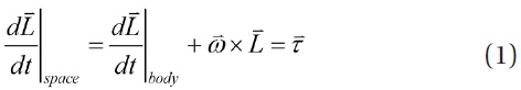
where
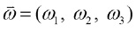
is the angular velocity of the rotating body. If external torque does not exist

then
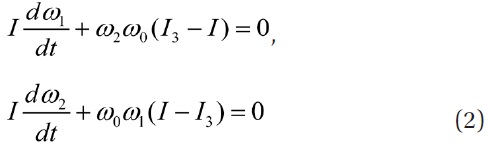
where
The coupled solution for

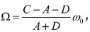
where Ω is defined as
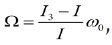
and the amplitude
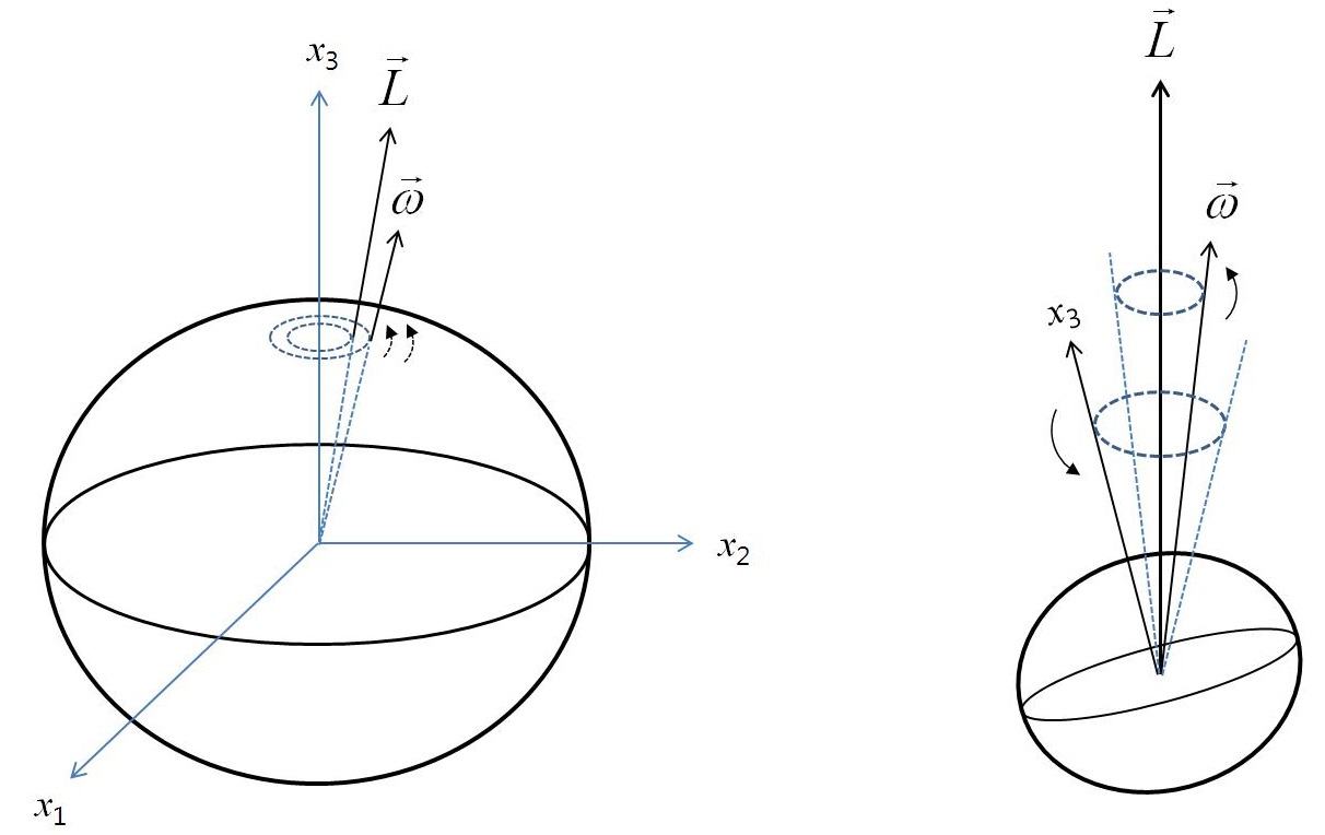
If the Earth were perfectly rigid, it should show this free wobbling motion with a frequency specified as
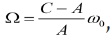
of which corresponding period is about 304 days. As the Earth rotates daily, an observer on the Earth should see that both the angular momentum and velocity vectors slowly encircle the
The Earth is not perfectly rigid but undergoes small amount of deformations due to various agitations. Denote the small variations in the inertia tensor, angular velocity, and angular momentum as

and , then terms for Earth’s spin rotation are defined as follows.
First, the inertia tensor
It is noted that
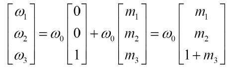
The angular velocity

is written as follows.
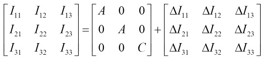
The angular momentum
in tensor form is given as
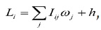
and its matrix representation is given as follows.
where the first order terms only are retained with neglecting much smaller second and higher order terms.
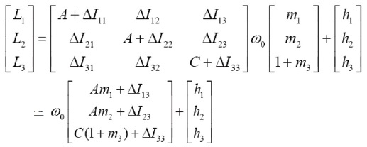
After a little algebra, three components of the governing equation for perturbed spin rotation of the Earth are found as follows.
Divide the first and second equations by
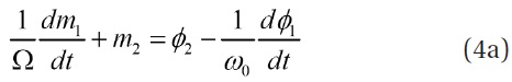
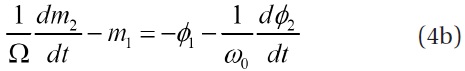
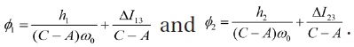
where the two excitation functions
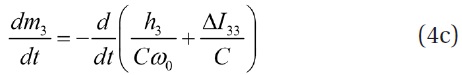
The third equation can be rewritten as
In case

The other case of Δ

Suppose a periodic variation in Δ
If the two excitation functions
Write periodic excitation as
Expression for Δ
where
In the fore part of this section, the free and forced wobbles of rotating rigid Earth were considered. Calculation of the Chandler wobble period for more realistic Earth model is not a trivial task. Chandler wobble frequency of elastic and oceanless Earth was acquired as
where
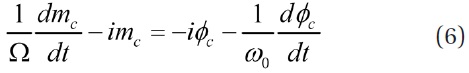
While Eq. (6) relates the excitation function and polar motion of rigid Earth, similar equation for realistic Earth is acquired by replacing the Chandler frequency with the following one;
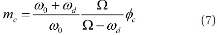
Formerly, the perturbation in Earth’s angular velocity and pole offset were considered to be the same with only difference in direction,
where
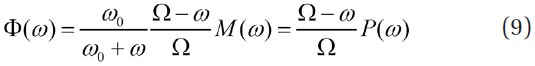
where Φ(
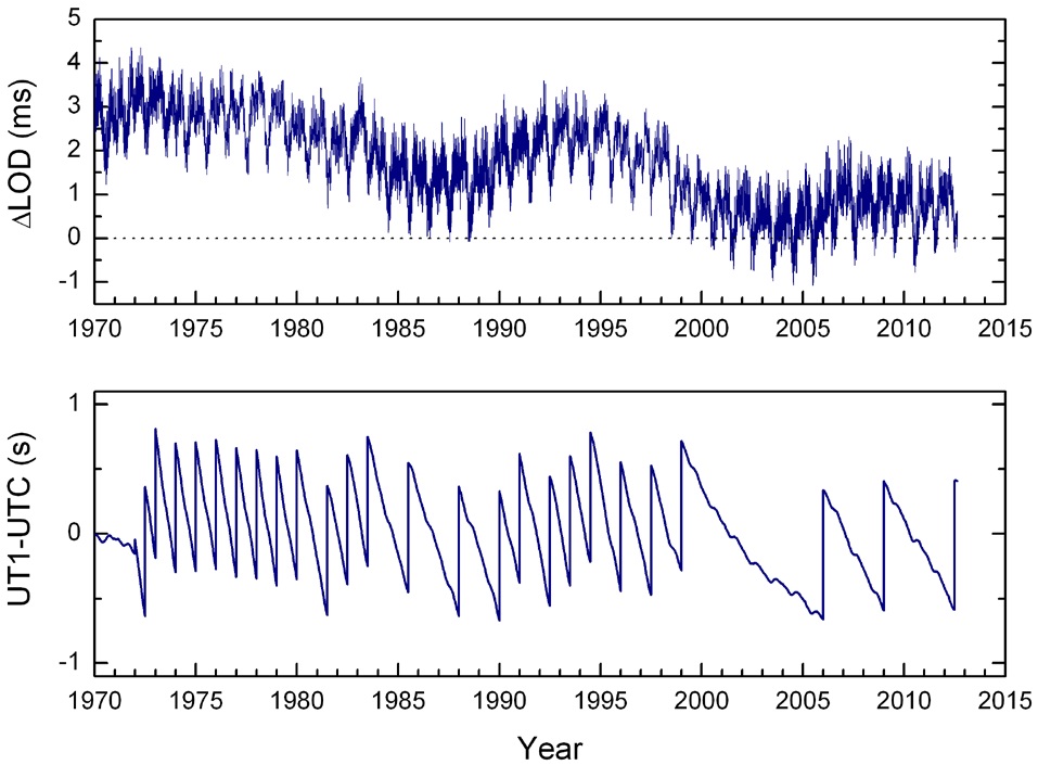
For this study, the most recent dataset of LOD and polar motion has been downloaded from the IERS website (http://www.iers.org/IERS/EN/IERSHome/). In Fig. 2, two time series of excessive LOD and UT1-UTC of IERS EOP 08 C04 (simply C04) since 1970 are illustrated. The dataset C04 has been produced as combined solution of VLBI, GPS, and SLR on daily basis and is generally regarded as the most reliable one. From the illustration, annual and decadal perturbations can be recognized easily (Fig. 2). The excessive LOD has been decreasing during the last forty years, which is the opposite trend of secular deceleration of the Earth. The cause of this decrease should be ascribed mainly to the tiny differential rotation in the Earth’s core associated with the geomagnetic field. This anomalous trend of LOD is also shown by leap seconds in the UT1-UTC time series, where the time interval between successive leap
seconds has been increasing.
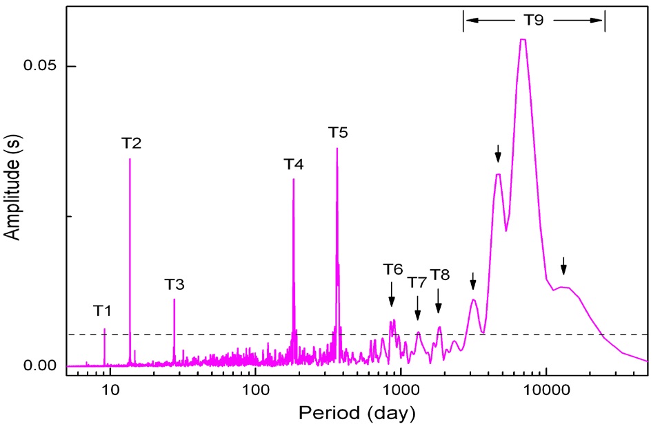
The Fourier amplitude spectrum of the excessive LOD time series was acquired by direct integration of the signal multiplied with sine/cosine waves for each frequency in time domain, and is illustrated in Fig. 3. As a pre-process, linear trend has been eliminated from the time series before spectrum evaluation. No filtering or other further treatment has been applied. Main features revealed on this spectrum are described as follows.
Six conspicuous peaks on the spectrum are marked as T1 - T5 and T9. These six periodicities are 9.13, 13.7, 27.6, 183, 365, and about 6900 days respectively. Other peaks over 95% significance level are marked as T6 - T8 or by arrows. The periods of T6 - T8 are roughly 852 - 893, 1320, 1840 days. Unlike the major peaks of lunar and solar origin, periodicities of the minor peaks cannot be clearly identified. Wide peak of long period marked as T9 is spread between 2830 and 23000 days, and its three split peaks are centered near 3170, 4650, and 13400 days respectively. Because there is no known atmospheric/oceanic perturbation of this period range (T9), main contribution for the wide T9 peak should come from the Earth’s internal process and the 18.6 year lunar orbital precession.
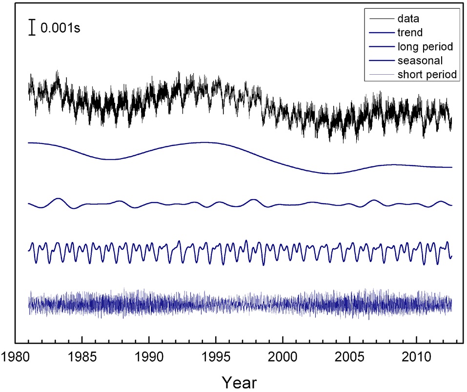
Separate time series of different period bands were acquired by using simple spectral windows in the frequency domain. They are illustrated as four curves together with the total signal (Fig. 4). Each spectral windows were set as unity for specified period only and zero otherwise; (i) T > 2000 days for decadal trend, (ii) 500 < T < 2000 days for long period, (iii) 100 < T < 500 days for seasonal, and (iv) T < 100 days for short period bands respectively.
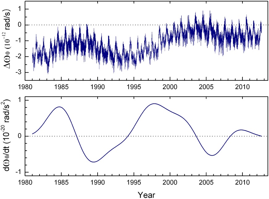
The Earth’s spin angular velocity and acceleration were calculated from the excessive LOD time series, and are shown in Fig. 5. The angular velocity is directly acquired from the raw data without any filtering, while only the
decadal trend was used to calculate angular acceleration with suppressing high frequency blow up. Due to the large and positive angular acceleration at the two periods; 1981 - 1987 and 1995 - 2003, Earth’s angular velocity has increased recently. Large decadal fluctuations exist in the Earth’s angular acceleration, as can be seen in the figure. Since this perturbation is of period of several years or longer, it cannot be an atmospheric/oceanic effect.
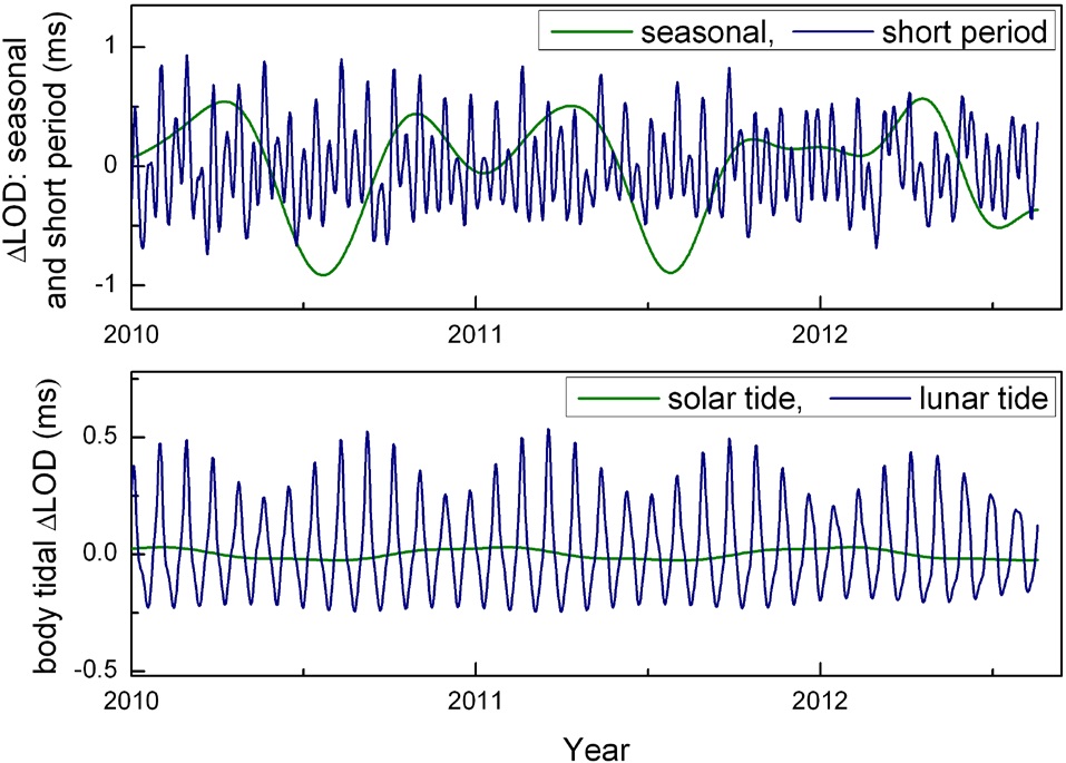
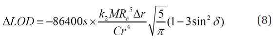
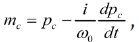
By using Eq. (8), the excessive LOD due to the lunar and solar body tides were calculated. For a time span, between Jan 2010 and Aug 2012, are illustrated in Fig. 6 together with
the seasonal and short period components of excessive LOD data. A good part of the monthly perturbation of LOD can be explained by the Earth’s body tidal deformation of lunar origin. However, the seasonal perturbation induced by solar body tide is much smaller than the observed data. The major part of this difference can be explained by seasonal changes in the global atmospheric circulation pattern.
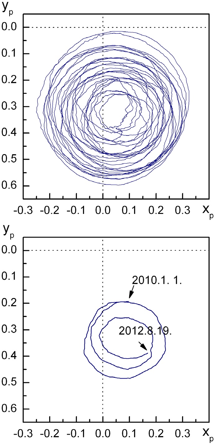
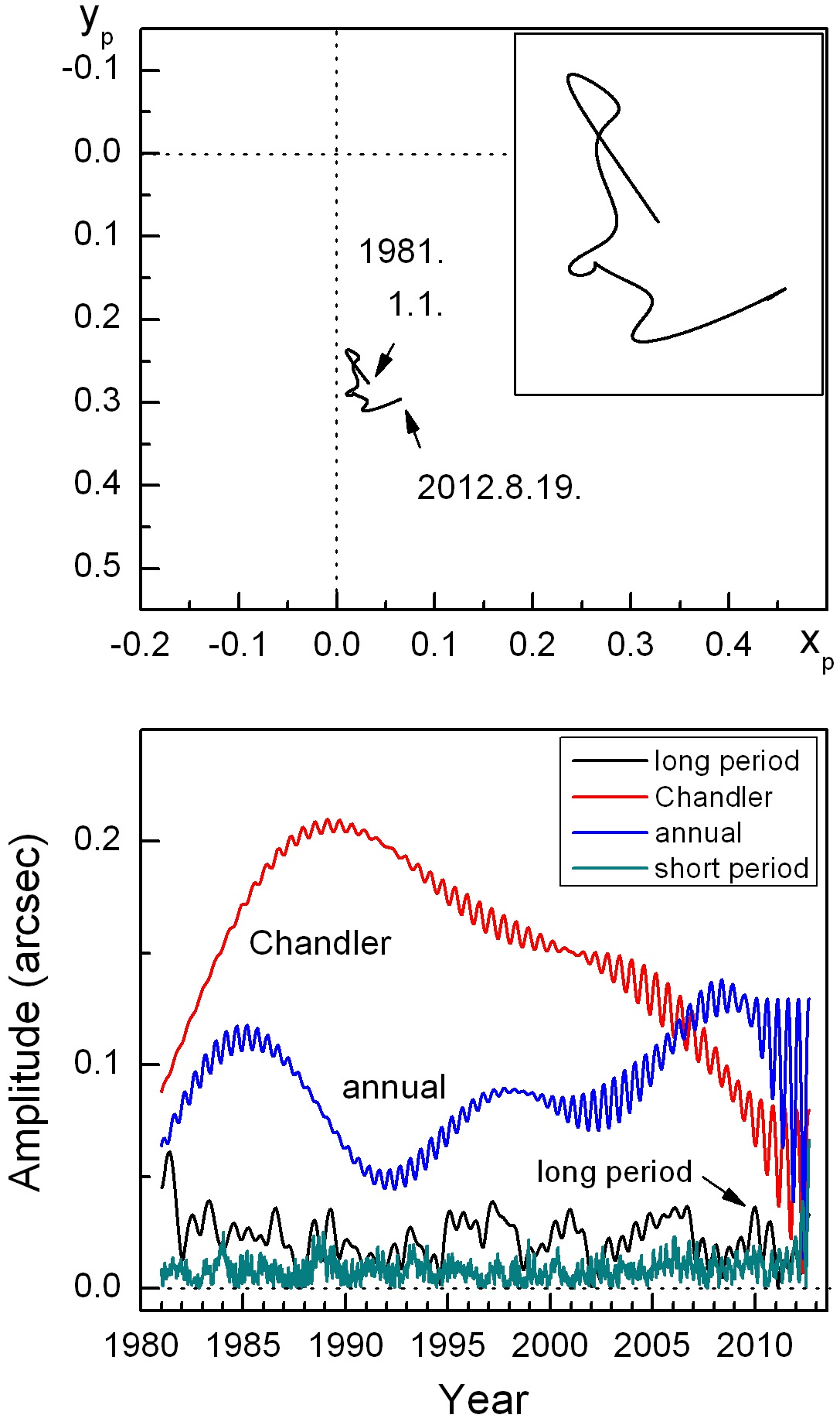
Two graphs describing the polar motion based on the IERS C04 dataset are shown in Fig. 7. The position of the origin (0, 0) of the graphs corresponds to the Reference Pole. The pole denoted by
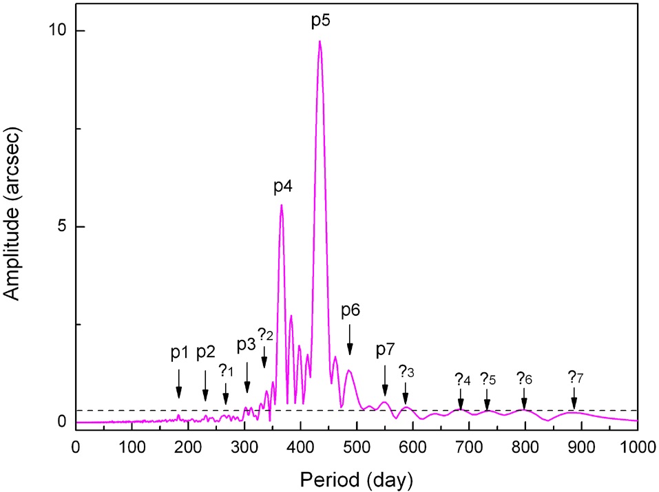
The Fourier spectrum of the polar motion data is shown in Fig. 8. This spectrum was acquired for the polar motion data of time span between Jan. 1, 1981 and Aug. 19, 2012. Fast Fourier transform was applied for the complex time series
significance level, and there are seven other peaks marked with question mark (?) with each index number, of which amplitudes are slightly over or below 95% significance level (their amplitude maxima periods are 260-266, 350, 587, 683, 734, 795, and 885 days). No known atmospheric/oceanic phenomena exist for these periodicities.
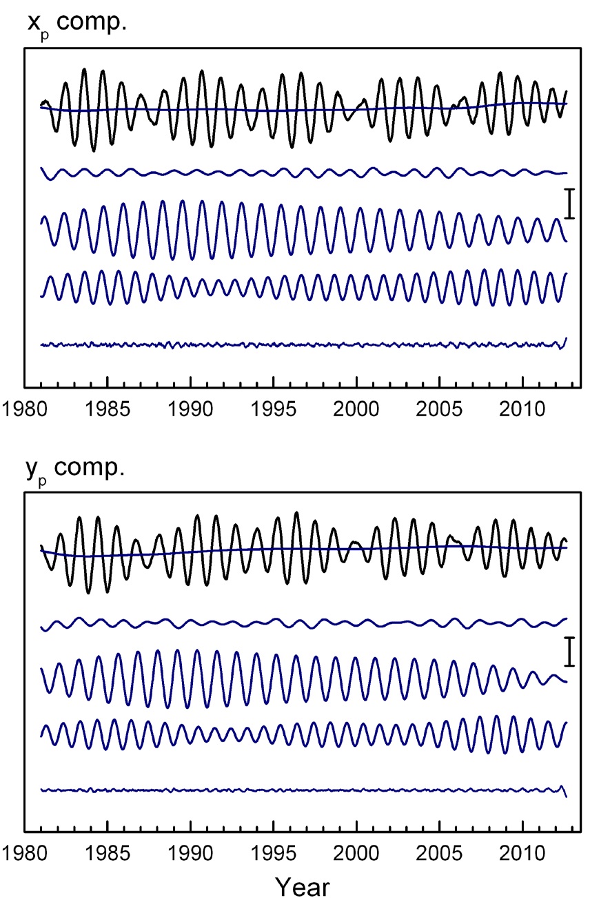
Five different period bands of the polar motion were acquired by flat spectral window in frequency domain and are shown in Fig. 9. These are the decadal trend (superposed on total component), long period, Chandler, annual, and short period components. The Chandler and annual components are the two dominant ones. However, their amplitudes are varying with time in certain amount. The short period component is composed of different periodic ones as, 300 day period, semi-Chandler, semi-annual,
The linear trend of the polar motion, called polar wander, was identified as 8.1 cm/yr to the direction of 59° W.
[Fig. 8.] Fourier amplitude spectrum of polar motion. The dotted line is the 95% significance level.
Excluded of this linear trend, the average pole (which should approximately coincide with the principal axis of the Earth)
shows drift of complicated feature, which is illustrated in Fig. 10 (top). The amplitudes of the four different band polar motions are shown together as four each time series (bottom). Variability of amplitudes of Chandler and annual wobbles can be recognized in Fig. 10, where the occasional oscillatory behaviors of the two main wobbles reflect that the two motions were elliptical at those times.
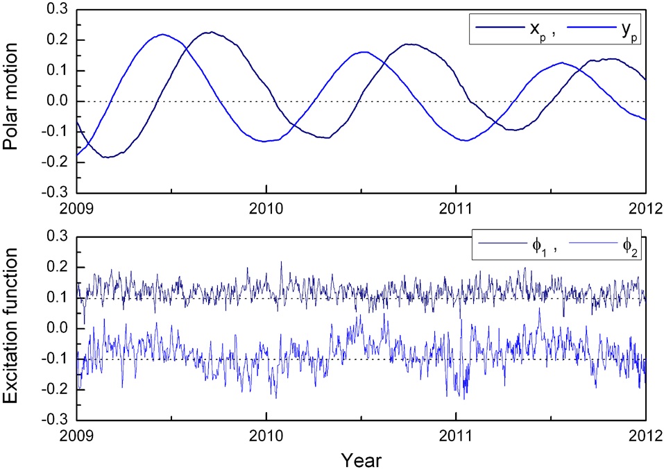
Two components of polar motion excitation function
Both the LOD and polar motion are composed of numerous different periodic components. While the overall features of the two were described in the former section, following aspects are discussed in this section; (i) decadal trend of LOD time series, and (ii) possible origin of 490-day period component of polar motion. Further studies are suggested as well.
Currently, average LOD is longer by a small amount than its nominal value, and has been decreasing through the last few decades. As noted earlier, positive angular acceleration existed at two time spans; 1981 - 1987 and 1995 - 2003, and recent Earth’s angular velocity has been increased accordingly. Average excessive angular velocity of the Earth since year 2000 is Δ
The observed recent change in the linear trend of pole drift is also noticeable, however it cannot be clearly interpreted either. Compared with the drift of last century ; 10.9 cm/yr to 79° W (Gross 2009), recent drift 8.1 cm/yr to 59° W is slower by 2.8 cm/yr and tilted by 20°. No single cause may be sufficient for this change, and both the internal and external processes of the Earth should all together be responsible. Again assessments of each processes including core/mantle motion and surface reformation of the Earth would be desirable. The recent pole drift might be affected by the recent vast glacier reduction in Greenland. Knowledge of elastic/viscoelastic response of the Earth due to loading/unloading is necessary in this regard.
Numerical experiment led positive evidence of the 490-day period signal in the Earth’s polar motion being a real component (Na et al. 2012). It is interesting that almost identical periodicity exists in different phenomena such as auroral occurrence, solar wind, and geomagnetic field (Silverman & Shapiro 1983, Richardson et al. 1994, and Ste?tik 2009). It should be rather surprising coincidence, if none of these 490 day or 1.3 - 1.4 year periodicity of the four aforementioned phenomena are not related with others. Here, the reality and its origin of the 490-day period polar motion are considered. First, it is claimed that the 490-day component is not another side robe such as those can be seen between the annual and Chandler peaks in the polar motion Fourier spectrum (Fig. 8). After comparison of calculated polar motion spectra by maximum entropy method both for the data and synthesized, they suggested 490-day period signal is more likely real signal than an artifact (Na et al. 2012). As can be seen in both the spectrum (Fig. 8) and the time series (long period component in Fig. 7), the amplitude of 490-day period signal is about 20 milliarcsec and bigger than other formerly recognized minor components; semiannual, 300-day period, semi-Chandler component. Inner-core wobble might be a candidate for the mode associated with the 490-day polar motion. However, it is discouraging to see that theoretical estimates of inner-core wobble period are longer as between 900 and 2500 days (Dehant et al. 1993, Rochester & Crossley 2009). On the contrary, those theoretical estimates could have been misled due to difficulties involving boundary condition or others. One may resort to the possibility of it being a driven oscillation by solar wind. This possibility is not large, because the mechanical momentum/angular momentum carried by solar wind flux passing near the Earth is not sufficiently strong. Finally, there may be an unknown mode of oscillation in the Earth associated with the anomalous region near the core-mantle boundary. More concrete and quantitative assessments about the aforementioned possibilities are desirable.
By using accurate ocean tide model and atmospheric circulation model, it is possible to calculate their excitations in LOD and polar motion. Fortnightly ocean tide and seasonal atmospheric wind pattern change should be the main causes of the excessive LOD of corresponding period ranges. Comparison of these excitation functions with the ones acquired directly from Earth’s rotation data as shown in Fig. 11 will enable further investigations. Some of this type researches have been reported in literatures, and more thorough ones will be accomplished, if more accurate and extensive observations on the geophysical processes be available.


![Polar motion and excitation function: two components of polar motion devoid of linear drift (above) and those of the excitation function calculated from them (below). Both units: [arcsec].](http://oak.go.kr/repository/journal/12056/OJOOBS_2013_v30n1_33_f011.jpg)