The use of generating functions for solving optimal rendezvous problems has an advantage in the sense that it does not require one to guess and iterate the initial costate. This paper presents how to apply generating functions to analyze spacecraft optimal reconfiguration between projected circular orbits. The series-based solution obtained by using generating functions demonstrates excellent convergence and approximation to the nonlinear reference solution obtained from a numerical shooting method. These favorable properties are expected to hold for analyzing optimal formation reconfiguration under perturbations and non-circular reference orbits.
For optimal formation reconfigurations of satellites in space, various analytical and numerical methods have been developed so far. Carter and Pardis analyzed for the optimal thrust which had the upper and lower limit (Carter & Pardis 1996). Palmer presented an analytic solution for the optimal reconfiguration problem based on the Fourier series expansion of thrust (Palmer 2006). Cho & Park derived a simple analytic solution for linear dynamics in the local vertical, local horizontal frame (Cho & Park 2009). Lee and Park derived approximated analytical solutions considering nonlinearities of the terrestrial gravity, eccentricities of a chief satellite, and J2 effects by perturbing the solution to the linear Hill equation (Lee & Park 2011). These analytical methods generally provide solutions based on the linear dynamics, which are limited to describe the actual dynamic environments precisely. While numerical methods can be employed to yield a precise solution based on nonlinear dynamics, it usually requires initial guess and iterative process for obtaining the initial costate vector accurately.
Recently, Guibout & Scheeres formulated a formation reconfiguration problem near the
In this paper, Park et al.’s nonlinear optimal control method with generating functions is applied to the optimal reconfiguration problem on the Projected Circular Orbit (PCO) to analyze the performance of the generating function approach comprehensively. The analysis is conducted on the convergence of trajectories and performance index to those of a nonlinear reference solution obtained from a numerical shooting method. The performance index analyses also exhibit some insightful characteristics by varying PCO configuration parameters under nonlinear dynamics.
2.1 Necessary conditions for optimal reconfiguration problems
An optimal reconfiguration problem for satellites flying in formation can be formulated as an optimal rendezvous problem, and can be mathematically framed as follows: minimize the performance index
subject to nonlinear dynamic equations in affine form with initial and final boundary conditions
where x ∈


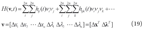
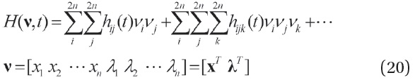
λ is the costate vector, and the subscripts on the bottom of Eqs. (4) and (5) indicate partial derivatives. When Eq. (6) is substituted into Eqs. (3)-(5), the optimal reconfiguration problem is expressed as a TPBVP for a standard Hamiltonian System.
Once the initial costate vector λ0 is obtained, this TPBVP is transformed into an Initial Value Problem (IVP), and the solution for optimal reconfiguration is obtained through a simple forward integration. When the dynamic system is nonlinear, many numerical methods can be used for obtaining the initial costate vector. However, it requires initial guess and iterative procedure for determining the initial costate vector, which may cause computational burdens to design optimal reconfiguration trajectories for various boundary conditions and time spans of formation flying.
2.2 Solution for optimal reconfiguration problems in terms of generating functions
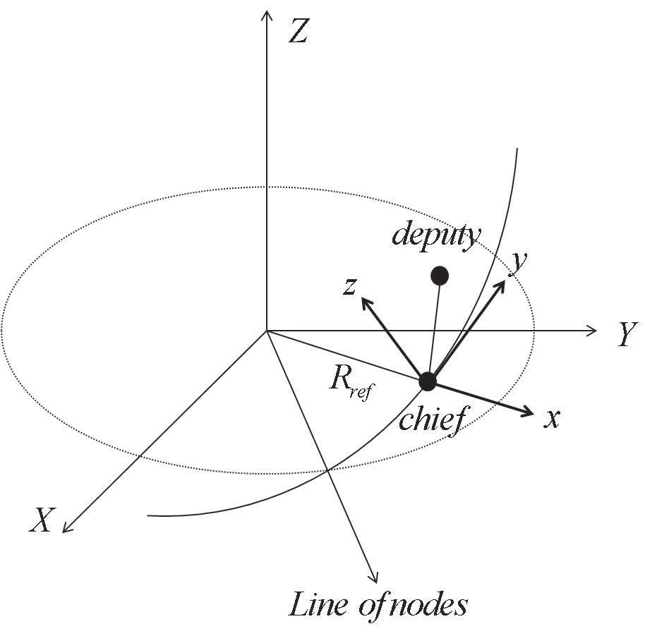
The nonlinear relative motion for optimal reconfiguration problems is expressed in the RSW coordinate system as shown in Fig. 1. The frame

in the RSW coordinate system as follows.
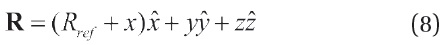

earth, the relative dynamic motion of the deputy with respect to the chief in the RSW coordinate system is stated as
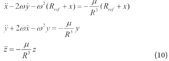
where
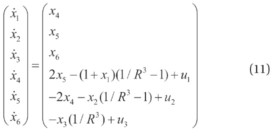
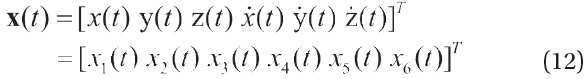
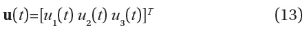
Here, [x1 x2 x3]
Now the optimal control method using the generating function is briefly summarized and applied to the optimal reconfiguration examples. The details regarding the generating function and the Hamiltonian system are given in Park et al. (2006) and Greenwood (1977). First, define another trivial Hamiltonian system for constant flows of initial state and costate vector as
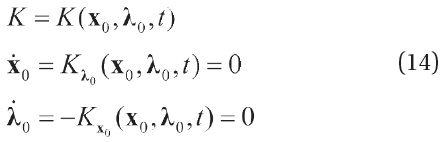
where
Theoretically, 2

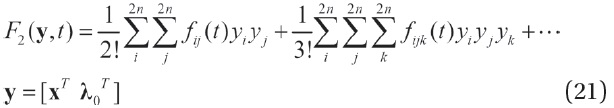
Each generating function satisfies the following relationships:
When the associated Hamilton-Jacobi equation, Eq. (17), is solved for the
In order to solve the Hamilton-Jacobi equation, the Hamiltonian is first expanded as a Taylor series with respect to a nominal solution as follows:
Here,
Next, the
The maximum order of the
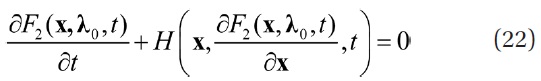
Balancing Eq. (22) for like kinds of variables results in the ordinary differential equation for the coefficients of Taylor expansion. It turns out that the initial condition

After introducing the boundary conditions for the reconfiguration problem, the initial costate vector and the performance index are expressed as follows (Park et al. 2006):
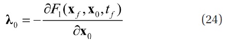

The steps up to Eq. (24) show that the optimal control problem can be converted into the IVP, not the TPBVP, without any iterative procedure for determining the initial costate. Eqs. (24) and (25) state that it is necessary to obtain the associated generating function only once. That is, the initial costate vector and performance index can be obtained by simply introducing the given boundary conditions into Eqs. (24) and (25). These characteristics can be advantageous in solving for a number of boundary conditions and time spans for multiple satellites in formation.
In order to demonstrate the convergence of trajectories and performance index based on generating functions to a nonlinear reference solution, the linear, second and third order solutions are developed by using our approach. The expanded generating function and their coefficients are obtained by the Mathematica-based HJ package developed by Guibout, which implemented all the steps from Eq. (14) to Eq. (23) (Guibout & Scheeres 2004). The nominal solution for obtaining the generating function is defined as 0 which is a trivial equilibrium solution of the RSW coordinate system. The initial costate vector satisfying the boundary conditions is determined from the
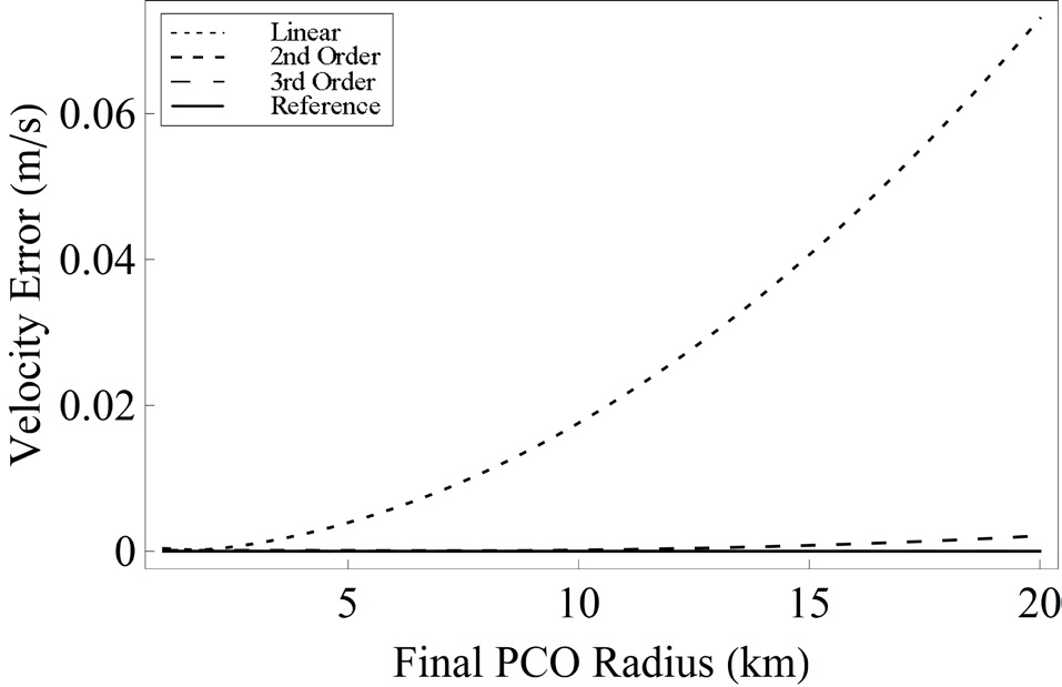
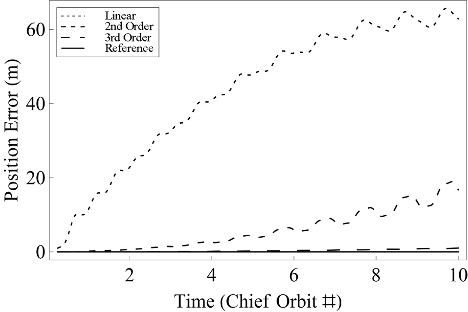
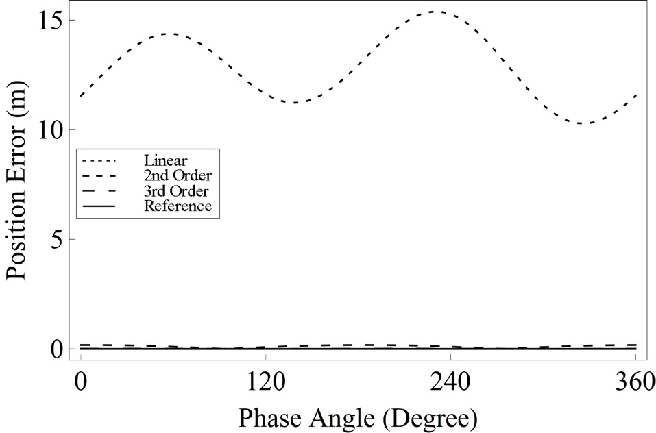
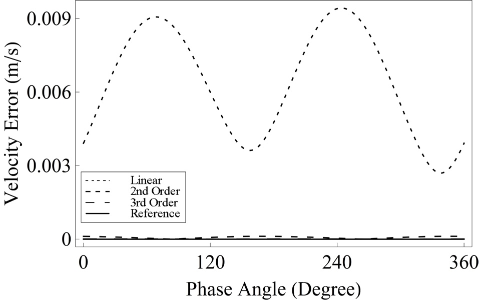
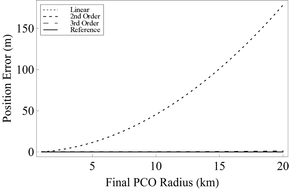
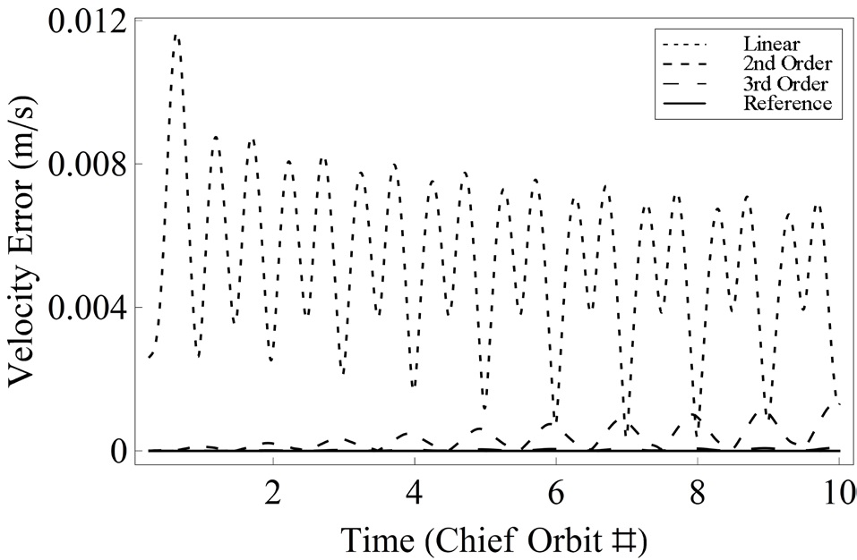
As a verification of the convergence of solution based on generating functions to a nonlinear reference solution, the satisfaction of the prescribed boundary conditions is tested through the error analysis. The linear, second and third order solutions based on generating functions are compared with the reference solution obtained from a numerical shooting method. For error analyses, the position and velocity vectors are considered separately, and are compared with prescribed terminal boundary conditions. In order to describe various formation reconfiguration examples, three cases are addressed as follows:
Case 1. Errors according to the change of ρf
Case 2. Errors according to the change of tf
Case 3. Errors according to the change of α
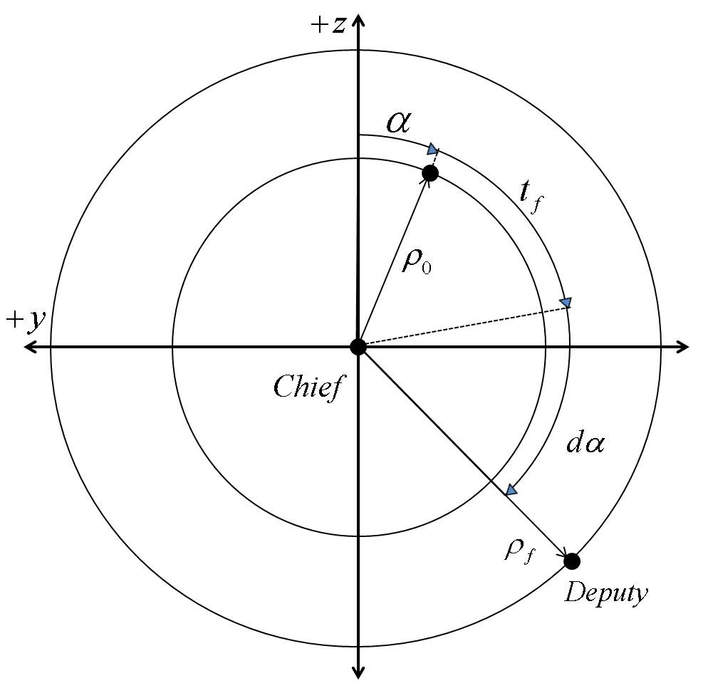
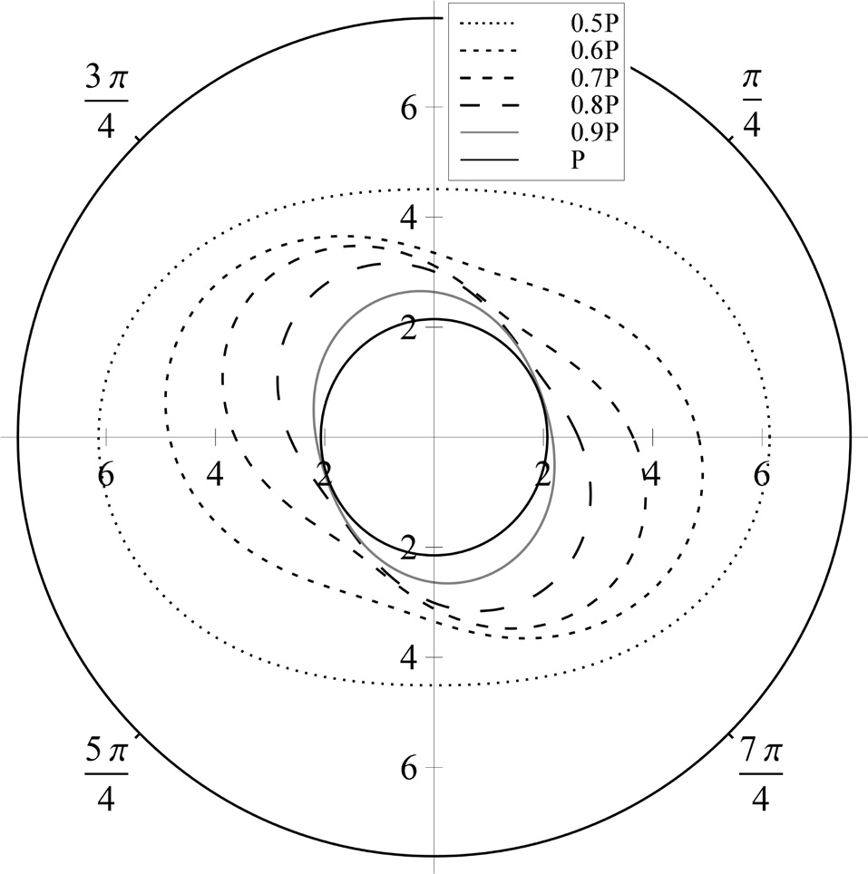
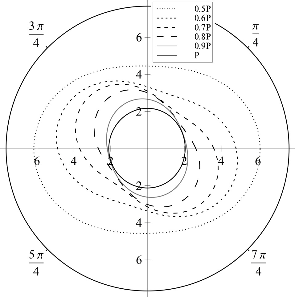
Fig. 2 represents the configuration parameters defining the boundary conditions on the PCO.
of the PCOs before and after reconfiguration, respectively.
where
The position and velocity errors for Cases 1, 2 and 3 are presented in Figs. 3-8, respectively. The fixed configuration parameters for each case are given as follows:


In Figs. 3 and 4, while the position and velocity errors of the linear solution steadily increase as
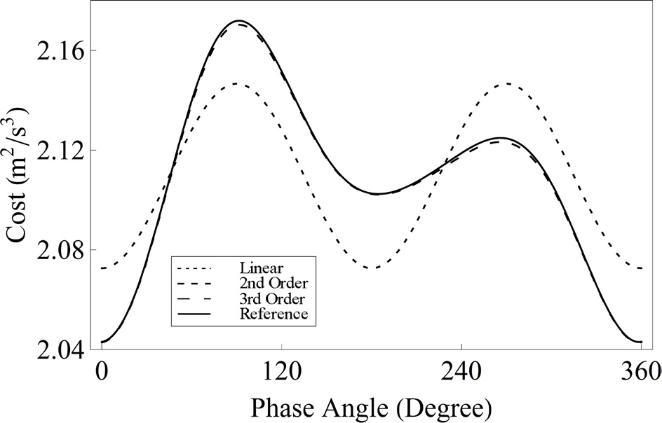
3.2 Analysis of performance index
In this section, the performance index based on generating functions is compared with that from a numerical shooting method. The performance index is displayed by varying the initial phase α and the operation time span
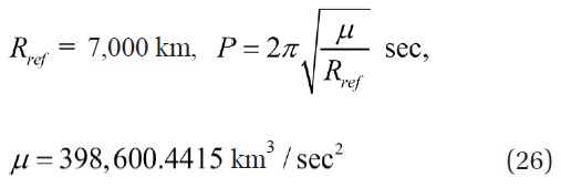
The period and radius of the reference orbit for all examples are defined in Eq. (26).
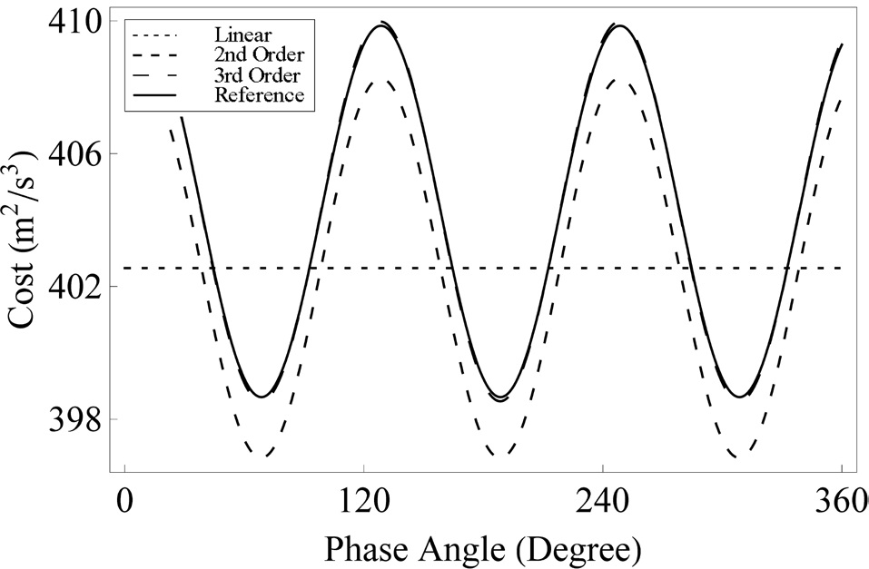
Fig. 9 shows the performance index variation according to the initial phase α with

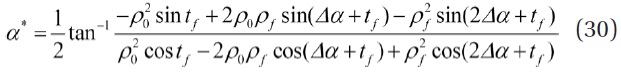
As shown in Fig. 9, the performance index variation by the initial phase α from the second and third order solutions are close to that from the numerical shooting method. Especially,rmance index of the third order solution approximates the numerical performance index quite closely. Fig. 9 allows us to analyze α* in the nonlinear dynamic system. Whereas two α*’s exist symmetrically in case of the linear solution, which can be confirmed by Eq. (30), only one α* has the minimum performance index in case of the second and third order solutions as well as the nonlinear reference solution.
Figs. 10-12 show the performance index variation by varying the initial phase α for a different transfer time
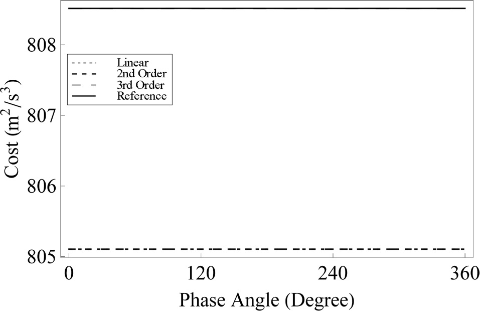
When a number of satellites maneuver on the PCO, it is often considered that satellites should be distributed uniformly
before and after reconfiguration for space interferometry. Figs. 13 and 14 show the sum of performance indices for three and six satellites that perform reconfigurations in equidistant intervals in terms of the initial phase α of the reference deputy satellite.
Other constant parameters are set as follows.

Figs. 13 and 14 show that the sum of performance indices of the third order solution properly approximates that of the nonlinear reference solution obtained from the numerical shooting method. Fig. 13 shows the case of three satellites performing the reconfiguration, in which only the sum of performance indices of the linear solution has a fixed value regardless of α of the reference deputy satellite; those of the nonlinear solution show periodic variations. Even though the boundary conditions in Eq. (32) represent big differences in the initial and terminal PCO radius, and thus possibly incur high nonlinearities of the central gravity field of the earth, Fig. 14 shows that for six satellites, the sum of performance indices in both the linear and nonlinear solutions always shows a fixed value regardless of α of the reference satellite. This phenomena turns out to be consistent, as long as the number of satellite is more than 6.
The optimal control problem for the formation reconfiguration on the PCO has been solved using the generating function. The higher-order solution obtained by using the generating
function converges to the nonlinear reference solution without any iterative procedure of obtaining the initial costate for the various boundary conditions in the nonlinear dynamic system. The semi-analytical performance index derived from the generating function closely approximates the performance index obtained from the direct numerical integration. It allows us to analyze performance index characteristics of the nonlinear formation reconfiguration, which shows distinct patterns from the linear reconfiguration. The analysis for the errors and performance indices demonstrate that the generating function approach is an appropriate method for nonlinear optimal reconfiguration of formation flying satellites. In the future, the generating function approach will be applied to more general case of perturbed elliptical reference orbit.