When many satellites flying in formation perform reconfiguration, they are subject to collision with each other. While it is possible to prevent the collision by immediately applying the thrust on detecting the risk of collision, it usually requires large fuel consumptions, and thus shortens mission life time (Katz et al. 2011). Thus it is more fuel-efficient to design a collision-free reconfiguration trajectory a priori, if possible.

Recently, many relevant studieshave been conducted. Sultan et al. (2006) suggested an algorithm optimizing the way-point using a gradient methodin the gravity-free, deep space. Schaft et al. (2006) demonstratedan algorithm using direct optimization method in free space. Min et al. (2010) solved the optimal control problem using the linear programming by reconstructing the Hill’s dynamics (Clohessy & Wiltshire 1960) as parametric expressions. Sauter & Palmer (2012) obtained the solution from the Model Predictive Control (MPC) using an analytic solution of optimal control problem under the Hill’s dynamics. Sun et al. (2012) tried to obtain the safe reconfiguration trajectories by redefining the Hill’s dynamics as a static model and employinga genetic algorithm.

This paper extends Sultan et al.’s method for collision avoidance reconfiguration algorithm for gravity-free, deep spaceinto that for a central gravity field near the Earth.Similarly in the case of Sultan’s algorithm forgravity-free space, way-points are introduced for collision avoidance and trajectories of satellites are represented by states of way-points. In order to generate the reconfiguration trajectories between neighboring way-points, the analytic solution of energy optimal control problem under the Hill’s dynamics is used. The optimal way-points which generate collision-free trajectories are found by a gradient method. Then, the obtained way-points and analytic solution generate the whole trajectories by connecting the subinterval reconfiguration trajectories. The proposed algorithm can develop safe reconfiguration trajectories and is easily applicable to the case of multiple satellites reconfiguration.

This paper is organized as follows. Section 2 describes parameterization of energy optimal control problem-performance index, equation of motion, boundary condition-with collision avoidance constraints using the state of way-points. Section 3 explains various optimization algorithms. Section 4 shows the result and interpretation of applying the algorithm to a simple collision avoidance example. The conclusion and the future works follow in Section 5.

A collision-free optimal trajectory can be estimated by solving the optimal control problem with collision avoidance constraints. In order to take account of the Earth’s gravitational effects, the circular unperturbed Hill’s dynamicsare incorporated. The optimal collision avoidance problem can be mathematically stated as follows:

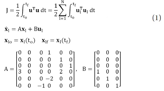
Eq. (1) represents the total performance index of N satellites in formation, which is simply a summation of integral- squared control of each spacecraft. x₁ and u₁ are state and control vector of l-th satellite and x and u are total state and control vector of entire satellites, respectively. Eq. (2) sets the distance limit between two satellites for collision avoidance in reconfiguration:

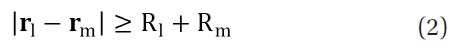
r_l is the position vector of l-th satellites and R_l is radius of buffer region centered on l-th satellite. If the distance between two satellites is smaller than the summation of two radii, these satellites are considered to collide. The summation of two radii is called the safe limit distance.

In order to apply the collision avoidance inequality constraints, the way-points are defined as the location which satellites must pass through (Sultan et al. 2006). The optimal way-points that do not cause a collision can yield collision-free optimal trajectories.

The trajectories between M+2 way-points including the initial and final positions can be estimated by using an analytic solution of optimal control problem with initial and final conditions. Eq. (3) is an analytic expression for the energy-optimal control problem satisfying rendezvous- type boundary conditions under the Hill’s dynamics (Lee & Park 2011). Note that it is a solution without collision avoidance constraints. As it is difficult to solve the energy optimal control problem directly with collision avoidance constraints, our algorithm begins with an initial analytic solution without collision avoidance constraints

where

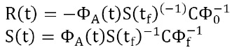
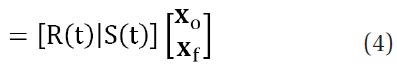
The analytic expression for optimal control can be factored into time-dependent terms and prescribed boundary conditions as in Eq. (4). By applying Eq. (3) to the Hill’s dynamics, the analytic trajectory of the energy optimal control problem with boundary conditions can be developed as

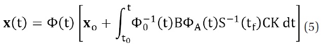
which can be also factored into a time-dependent function and prescribed boundary conditions.

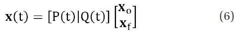
where

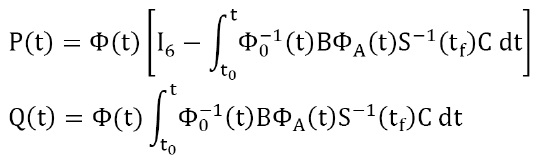
Eqs. (4) and (6) are analytic solutions for the whole time interval [t₀, t_f ]. Likewise, analytic solutions between neighboring j-th and (j+1)-th way-points can be estimated. With the j-th and (j+1)-th way-points as initial and final conditions, the optimal state and control trajectories can be expressed as

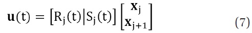
If these analytic solutions for the time interval [t_j, t_j+1] are applied and linked to all way-points, the solution for the entire time span [t₀, t_f] can be calculated.

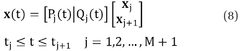
In Section 2.1, the states of way-points are defined as x. Two additional variables are also defined. U is a variable for M+2 way-points of entire satellites:

The initial and final conditions of each satellite are given in U. M way-points of entire satellites which excludethe boundary conditionsare combined into the vectorz, which is introduced for collision avoidance algorithm:

With these variables U and z , the performance index and collision avoidance constraints can be stated as

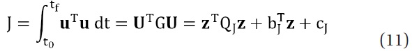
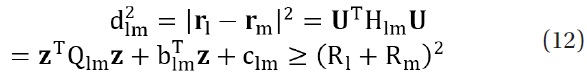
Q_J, b_J, c_J, Q_lm, b_lm, c_lm are founded by reconstructing G and H_lm with boundary conditions and M way-points. As the algorithm is described in Section 3, the performance index and collision avoidance constraints, which are represented as variables, create the optimal variables that do not incurcollision.

The unconstrained solutions between two way-points are first obtained from the analytic solution of energyoptimal control problemby Lee & Park (2011) as the initial solution of the problem with collision avoidance constraints:

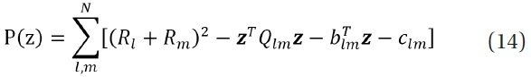
If the distances between satellites are smaller than the safe limit distance, satellites are considered to collide and violate the collision avoidance constraints. At this time, calculate the difference between the square of safe limit distance and the square of minimum distance between colliding satellites and define the penalty function P(z) as the sum of satellites violating collision avoidance constraints.

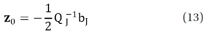
When the penalty function, which is described as the variable z, is positive, some collision arises. That means that the variable z which makes penalty function less than or equal to 0is the solution that does not cause collisions. Thus, when some satellites violateconstraints, update the variable z repeatedly using a gradient method to make penalty function negative or 0 by Eq. (15):

When the updated z satisfies the collision avoidance constraints, the next process is to determine the variable minimizing the performance index. Because the performance index J(z) is a function of variable z, update z again using a gradient method to minimize J(z) according to Eq. (16).

The final solution going through the upper two steps satisfies the collision avoidance and minimizes the performance index at the same time (Sultan et al. 2006). This solution is a set of states of way-points. Therefore applying the calculated state to Eqs. (7) and (8) and connecting reconfiguration subinterval divided by way-points generate the collision-free reconfiguration trajectories for the entire maneuver time. The gravitational field is incorporated as the coefficient matrix R_j(t), S_j(t), P_j(t) and Q_j(t), and are estimated from the Hill’s dynamics.

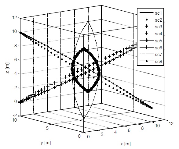
This paper focuses on developing a collision-free reconfiguration algorithm under the Hill’s dynamics without perturbation. Thus, the ‘swapping cube maneuver’ simulation, identical with the simulation in Sultan et al. (2006), is conducted to objectively verify the algorithm.

The total of 8 satellites are initially placed on each vertex

of a cube whose side length is 10 m, with one vertex located on a circular reference orbit of 700 km in altitude. Then each satellite swaps their position diagonally during 740.80 s.

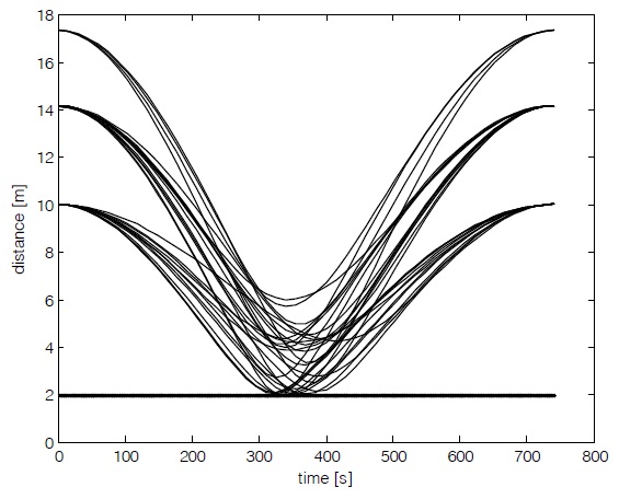
Fig. 1 shows the relative trajectories without collision avoidance constraints. Whether collisions may or may not occur can be observed by checking distances between satellites. Here the radius of buffer region is 1 m and the safe limit distance is 2 m. Without collision avoidance constraints, distances between satellites under the safe limit distance take place 12 times in 370.50 s from the start of reconfiguration (Fig. 2).

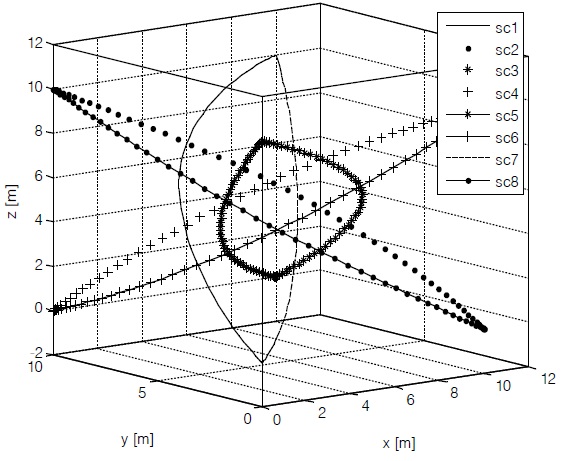
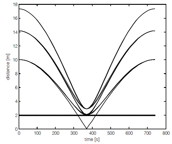
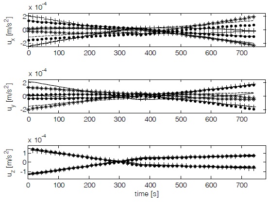
To prevent such collisions, the algorithm described in Section 3 is applied. Distances between satellites must be larger than the safe limit distance of 2 m. Fig. 3 shows the relative trajectories, and Fig. 4 shows the time history of relative distances after applying collision avoidance

constraints. Fig. 4 confirms that the resultant relative trajectories are safe reconfiguration trajectories without collisions. Fig. 5 shows time histories of control on each axis when there are collision avoidance constraints. While the performance index is 4.3679 × 10^-8 m²/s⁴ without considering collision avoidance, the performance index is 4.7869 × 10^-8 m²/s⁴ with collision avoidance constraints. The performance index increases by 9.5636% for 8 satellites and 1.1955% for each satellite by average to avoid collision.

A collision-avoidance reconfiguration algorithm under the Earth’s gravitational field has been developed by extending a collision-free reconfiguration method in gravity-free space. In

the algorithm, the way-points from analytic solution of energy optimal control problem under the Hill’s dynamics without collision avoidance constraintswere introduced as the initial solution of the constrained problem. Then, the collision- freestates and controls were developed, while minimizing the performance index. Through a simple simulation, it was confirmed that safe, collision-free trajectories was able to be generated for the linearized central gravitational field. The energy consumption for collision avoidance is minimized by trying to minimizethe distances between satellites. Because the way-points are introduced as variables, the dimension of collision avoidance constraints is restricted. It makes the algorithm useful in applying to a large group of formation flying.

As the Hill’s dynamics does not exactly represent the nonlinear gravity fieldnear a central body, it is necessary to extend the proposed approach into more general dynamic environments where a reference orbit is elliptic and possibly includes a variety of perturbations.