Various scheduling policies for real-time multiprocessors systems have been constantly evolving. Scheduling of real-time applications/tasks on multiprocessor systems often has to be combined with task to processor mapping. With the current design trends moving towards multicores and multiprocessor systems for high performance and embedded system applications, the need to develop design techniques to maximize utilization of processor time, and at the same time minimize power consumption, have gained importance. General design techniques to achieve the above goals have been fueled by the development of both hardware and software solutions. Hardware solutions to minimize power and energy consumption include: dynamic voltage and frequency scaling (DVFS) processors, dynamic power management modules (Advanced Configuration and Power Interface, ACPI), thermal management modules, intelligent energy management (IEM), and heterogeneous multicore or multiprocessor systems [1]. Software solutions for maximizing processor utilization and energy minimizations include: parallelization of instructions, threads, and tasks; effective thread/task scheduling; and mapping algorithms for multicore and multiprocessor systems.
In this work we propose a new energy aware, probability- based offline scheduling algorithm of aperiodic realtime tasks for a multiprocessor system. The proposed solution combines the traditional mapping and scheduling algorithm into a unified process. The proposed algorithm is modeled for multiprocessor (homogeneous processors) systems that support dynamic voltage scaling (DVS) processors. The algorithm is based of the force-directed scheduling (FDS) algorithm [2], most commonly used during the high-level design synthesis. The algorithm determines an optimal schedule for each task, on a processor operating at a discrete voltage level with constant frequency, which will be able to satisfy the deadline. The algorithm also maximizes the utilization of all processors, and minimizes the energy consumption of the system. For comparison purposes, this work implements four different variations of the scheduling algorithms for multiprocessor systems that support DVS processors. The first three scheduling algorithms implement the scheduling and mapping algorithms as different processes. The first scheduling algorithm, called scheduling after scaling (SaS), performs the mapping of tasks to the processors, and iteratively scales down the voltage of the processors from the maximum operable voltage, based on the slack of the tasks. Once the tasks have been mapped to the processors, voltage levels are determined, and scheduling is performed. In the second scheduling algorithm, called scheduling before scaling (SbS), the tasks are first scheduled based on the deadline (earliest deadline first, EDF) [3]. The SbS scheduling algorithm is similar to the lowenergy EDF algorithm proposed by Manzak and Chakrabarti [4]. Once scheduled, the tasks with slack are assigned to processors with lower operating voltages. In the above two algorithms, processors are added to the system, to satisfy the dependency and deadline constraints. In the third scheduling algorithm, called probability based scheduling (PbS), the scheduling is based on optimizing the probability (probability of utilization) of the tasks executing in a unit time step. The probability function optimizes the utilization of each processor, and hence the utilization of the whole multiprocessor system. Mapping of the tasks and assignment of voltage levels to processors is achieved by determining the probability of utilization of each processor operating at different voltages. The final scheduling algorithm, called energy-probability based scheduling (E-PbS), combines the process of scheduling, and mapping or assignment of voltages to processors, together. The probability of utilization function incorporates the energy factor, and the scheduling algorithm determines task operation times and voltage levels of the respective processors. The developed algorithms have been implemented, simulated and evaluated for synthetic real-time applications (standard task graphs). The algorithms are compared for utilization of the processors, number of processors (resources), and energy consumed by the processors.
Scheduling algorithms have been classically categorized into online or offline, priority or non-priority, pre-emptive or non pre-emptive, and hard or soft deadline scheduling algorithms. Two of the classical scheduling algorithms for uniprocessor are fixed priority rate-monotonic scheduling (RMS), and dynamic priority EDF algorithms [3]. With the advent of multicore and multiprocessor systems, where each processor is capable of dynamic performance and energy consumptions based on variable voltage and frequency operations, scheduling and mapping algorithms to optimize performance and energy have gained importance. Weiser et al. [5] were the first to propose the DVFS technique. Their approach was to reduce CPU ideal times, by dynamically adjusting DVFS levels in OS-level scheduling algorithms. Yao et al. [6] and Ishihara and Yasuura [7] proposed an optimal offline-scheduling algorithm for independent and dependent tasks, respectively, to minimize energy consumption.
Aydin et al. [8] proposed a dynamic speculative scheduling algorithm, by exploiting slack times. Zhu et al. [9] proposed scheduling algorithms to improve the above algorithms for multiprocessors for dependent and independent tasks, to share slack times. More recent works [10-14] on DVFS do not account for frequency scaling, as analysis shows performance loss on processor frequency scaling. Also, work by Dhiman and Rosing [14] has shown that memory intensive tasks have less dependency on frequency scaling, which is true with modern embedded applications. Also, issues such as task granularity and shared resource contention in caches, memories and buses have to be accounted for. Algorithms for resource contention aware or mitigations have been explored in [15-18]. Lee and Zomaya [19] proposed a DVFS energy aware scheduling algorithm for a heterogeneous distributed multiprocessor system. Also, work comparing dynamic power management and DVFS methods has been conducted by Cho and Melhem [20], and has concluded that DVFS scheduling methods provide better energy saving for multiprocessor systems. Shin and Kim [21] have considered the problem of mapping the tasks of the task graphs from real-time applications to available cores, and then determined the DVFS for each core to meet the timing deadlines, while minimizing the power consumption. The problem of determining the optimal voltage schedule for a real time system with fixed priority jobs, implemented on a variable voltage processor, is discussed in [22].
Okuma et al. [23] addressed the problem of less energy consumption, by simultaneously assigning the CPU time and a supply voltage to each task that results in low power. This algorithm uses a variable voltage processor core to schedule the tasks [7]. An online energy aware algorithm for distributed heterogeneous hard real-time systems, based on a modification of the EDF algorithm, is proposed in [8]. The energy reduction is obtained by reducing the speed of the processor when the only ready task in the system has no successor, or when the previous task has not exhausted its worst-case execution time (WCET).
In this work, we present an offline dynamic voltage scaling scheduling algorithm for dependent and non-periodic task graphs, to optimize energy consumption on a multiprocessor system. The proposed work in this article follows a similar approach to the method presented in [21], but with the following differences and advantages: 1) this work considers task graphs derived from real-time applications, as well as synthetic task graphs; 2) the process of mapping the tasks to a processor, voltage scaling of the processor and scheduling are considered together; and 3) only voltage scaling is considered in this work, for the reasons mentioned above. However, frequency scaling can also be implemented, by considering an appropriate cost function.
Definition 1 (Task model). A task model is required as the basis for discussing scheduling. A real-time task is a basic executable entity, which can be scheduled; it can be either periodic or aperiodic, with soft or hard timing constraint. A task is best defined with its main timing parameters. This model includes the following primary parameters.
ri - release time of the task
ei - WCET of the task
Di - relative deadline of the task
di - absolute deadline of the task
pi - period of the task
gi - start time of the task
hi - end time of the task
si - slack of the task = di ? ei
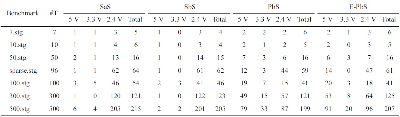
Definition 2 (Scheduling model). For the problem of scheduling, we consider a task set or application A = {T0, T1, …, Tn} = {Ti}, where each task Ti is an aperiodic task with a hard deadline di, and WCET of ei and best-case execution time (BCET) of ez. These tasks execute on a multiprocessor system consisting of processing elements PE = {PEj} = {PE0, PE1, …, PEm}, which can operate at a prespecified set of voltages V = {V1, V2, …, Vp}, where i < j implies Vi > Vj. We denote a task Ti running on the processor PEj scaled at voltage Vk as Tik. In this work we also phrase the WCET of a task Ti as its execution time at maximum voltage V1, denoted by ei1. Thus, its execution time at voltage Vk is determined as:

Also, all tasks T are subject to precedence constraints, and a partial order Ti < Tj is defined on T, where Ti < Tj implies that Ti precedes Tj. The problem of scheduling of an application A is denoted as:
If there exists a precedence operation between any two tasks, such that the execution of a task Ti should occur before the execution of task Tj, represented as Ti < Tj, then for each Ti ∈ T, ti + ei ≤ di and tn + en ≤ D, where D is the absolute deadline of the last task.
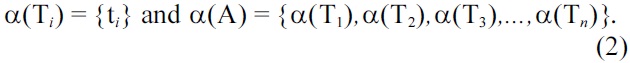
Definition 3 (Mapping and voltage scaling). Mapping is the process of assigning each task in an application to a processor, such that the processor executes the task and satisfies the task deadline, as well as other constraints (power, throughput, completion time), if any. For an application A = {T1, T2, …, Tn}, where Ti is a task instance in the application, mapping a task, denoted as σ(Ti), is defined as an assignment of the processor {Pj} = {PE1, PE2, …, PEm} = PE for the task Ti:

Application mapping is defined as mapping of all tasks, Ti, in the application A to processors, and is denoted as:

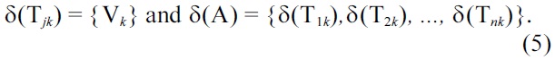
Voltage scaling is the processes of assigning a discrete operating voltage to each processor, such that the processor executes the tasks and satisfies the task deadline, as well as other constraints (power, throughput, completion time), if any. For a set of processors PE = {PE1, PE2, …, PEm} that can be scaled at discrete voltages V = {V1, V2, …,Vp}, voltage scaling is denoted as δ(Tik), and is defined as an assignment of voltages (Vk) and task (Ti) to the processors:
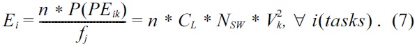
Definition 4 (Processor power model). Assuming that a processor PEik is scaled at a supply voltage Vk, and a frequency fj, and a task Ti takes ‘

where, CL is the output capacitance, and Nsw is the number of switches per clock. Energy consumption by a task Ti can be computed as:
From the above equations, we can conclude that lowering the supply voltage drastically reduces the power and energy consumption of the particular processor. The supply voltage also affects the circuit delay. The circuit delay is given by Td = k * Vk2/(Vk ? Vt)2, where k is a constant that is dependent on output capacitance, and Vt is the threshold voltage.
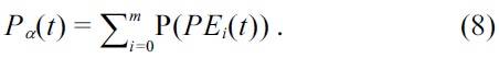
Definition 5 (Scheduling power and energy model). The power consumed by a schedule is the total power consumed by all tasks that execute at the time period t, and is denoted as Pα(t),
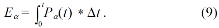
Energy consumed by the schedule is the integral of Pα(t),
Definition 6 (Problem statement). Given an application A with tasks Ti, determine an optimal schedule α(A) with minimal energy consumption for a multiprocessor system PE, while mapping tasks to PEs, σ(A) and voltage scaling the processors, δ(PE) in a multiprocessor system, such that all tasks are executed before their respective deadlines, and the end task before the final deadline D.
IV. ENERGY AWARE SCHEDULING ALGORITHM
Since the input task graph considered has only a final hard deadline, the first step is to determine the deadlines of all the tasks.
Find the path with the highest execution time: the path with the highest execution time is determined using a depth first search algorithm that determines all paths, from source to sink, of the task graph. The highest execution time is denoted as emax.
Find the deadlines of the tasks by backtracking: the deadlines of all the tasks are determined by backtracking to each task from the sink task. In order to determine the efficiency of the proposed algorithms the highest execution time emax is relaxed to ?max (D = ?max). This relaxation of the deadline allows the tasks to be operated at a lower voltage, and hence better power and energy consumption.
The deadlines of all other tasks are found by backtracking from the sink task. The deadline of a predeccessor task di with one sucessor task dj is determined as di = dj-ej. If a task has more than one successor, then the deadline is obtained by choosing the minimum of the differences of the deadlines and execution times of the successors. For example, a task i has successors j, k and l, then di is given, determined as min(dj-ej, dk-ek, dl-el). The slack of each task is calculated as the difference of deadline and execution time of each task, si = di-ei.
>
B. Scheduling after Scaling Algorithm (SaS)
The proposed SaS algorithm first allocates voltages to each task, and then progressively schedules and binds the tasks to the processors.
Step 1 (Scaling the voltage of each task). Assume that the tasks can only execute at a pre-specified set of voltages, and all tasks are by default assigned the highest voltage. First the tasks are sorted with respect to their slack. Then the task with least slack is made the current task (
Step 2 (Assigning the tasks on processors). The tasks are then scheduled on the processors, based on the EDF scheduling algorithm, and the first come first served (FCFS) mapping algorithm. At every instance of the start time of a task, a check is done to see if any processor is idle. The task is scheduled on the idle processor, if any; else a new processor is initialized. The pseudocode of the SaS algorithm is shown in Algorithm 1.
Algorithm 1 Scheduling after Scaling (SaS)
Inputs: A = {T1, T2,…, Tn}, PE = {PE0, PE1, …, PEm}
Outputs: σ(A), δ(Tik), α(Ti)
repeat {
assign highest voltage to tasks;
sort tasks based on their slacks;
scale voltages based on slacks;
} until (all tasks are scaled)
repeat {
schedule tasks based on deadlines (EDF);
assign tasks to free processors;
} until (all tasks are scheduled)
>
C. Scheduling before Scaling Algorithm (SbS)
This algorithm performs scheduling of the tasks on the available processor, before scaling the task voltages. This algorithm is an extension of the EDF algorithm. The SbS algorithm first performs scheduling, followed by assignment of voltage to the tasks.
Step 1 (Sorting the tasks). This algorithm is different from the SaS algorithm in sorting the tasks. All the tasks are initially sorted with respect to their deadlines (similar to EDF scheduling algorithm).
Step 2 (Scheduling of tasks). The SbS algorithm proceeds from the source task to the sink task. A breadthfirst search approach is adopted, to determine the task with the shortest deadline, and is scheduled first. This process is repeated, until all tasks are scheduled.
Step 3 (Assigning the tasks to processors). The tasks are then scheduled on the processors. At every instance of the start time of a task, a check is done to see if any processor is idle. The task is scheduled on the idle processor, if any; else a new processor is initialized.
Algorithm 2 Scheduling before Scaling (SbS)
Inputs: A = {T1, T2, …, Tn}, PE = {PE0, PE1, …, PEm}
Outputs: σ(A), δ(Tik), α(Ti)
repeat {
assign highest voltage to tasks;
sort tasks based on their deadlines (EDF);
assign tasks to free processors;
} until (all tasks are scheduled)
repeat {
for each processor {
for each task {
scale voltages of based on slacks and deadline;
} }
} until (all tasks are scaled)
Step 4 (Voltage scaling of the task on processors). The schedule produced from the above step is based on task deadlines only, and results in the minimum number of processors required to execute a task set. After scheduling, the voltages of the tasks are scaled, as in the SaS algorithm. The algorithm proceeds by sorting the processor, based on the tasks assigned to the processor. Voltage scaling is performed for each task on the processor. As voltage scaling is preformed on each task, the start and end times of its successor task in the same processor and any other processor, and the subsequent tasks on the same processor, are also modified. The pseudocode of the SbS algorithm is shown in Algorithm 2.
>
D. Probability based Scheduling Algorithm to Maximize Utilization
The proposed PbS algorithm increases the utilization of the processors, by optimizing the number of processors and energy consumed by the processors, by voltage scaling the tasks (Ti) that execute in the processor. The schedule is divided into equal time steps (Δtj). The PbS algorithm determines the probability of utilization P(Ti(Δtj)) of a task in each time step (Δtj). A task is scheduled to a time step where the probability of utilization of the task is maximum. The probability of utilization is the sum of the probabilities of utilization of the current task (Ti) and its successors (Tk). Initial probabilities are calculated by assuming all tasks are operating at the highest voltage. When voltage scaling is performed on the tasks, the probability of utilization is dynamically updated, based on the time steps assigned to the voltage scaled task. Finally, the number of processors required to execute the final schedule is calculated. The following steps explain the algorithm in detail.
Step 1 (Determining the time step). All the tasks in the task set A = {T1, T2, …, Tn} are assumed to be executing at their BCET, i.e., all the tasks are currently running at the highest voltage. Divide the task graph into time steps, with the smallest execution time of all tasks as the unit of time steps.
Step 2 (Best-case time scheduling). The next step is to perform the best-case time (BCT) scheduling algorithm. The BCT algorithm starts with the source tasks in the task graph, and proceeds in a breadth-first order. Each task is scheduled in the earliest available time step (BCT(Ti)), and only if its predecessors are scheduled. A task Ti is characterized by its start time, BCTg(Ti), and end time, BCTh(Ti). This algorithm determines the earliest possible execution time of the task graph.
Step 3 (Worst-case time scheduling). The worst-case time (WCT) scheduling algorithm works exactly in the same way as the BCT algorithm, except that it starts at the sink of the task graph, and proceeds upwards. This algorithm determines the longest possible execution time for the task graph. A task Ti is characterized by its start time, WCTg(Ti), and end time, WCTh(Ti). This algorithm determines the latest possible execution time of the task graph.
Step 4 (Determining the bound limit). The algorithm proceeds by determining the bound limits (Δti) of each task. The bound limit of a task Ti is calculated as:

where Δti represents the time steps within which the current task can be scheduled.
Step 5 (Determining the probability of utilization of each task in each time step). The next step in the algorithm is to determine the probability of utilization of each task in each time step, within the bound limit of the task (Δtij). The probability of utilization of a task Ti in a time step Δtij is represented as PU(Ti(Δtij)), where Δtij ranges from the earliest start time, to the latest end time of the task Ti.
Step 6 (Distributed probability of utilization). The distributed probability of utilization is the summation of probabilities of utilization of each task in each time step. It signifies the portion of a task that will be executed in a time step. The distribution probability of utilization DPU(Δtij) for a time step Δtij is given as:

Step 7 (Schedule the task in a time step). The algorithm schedules the task Ti at time step Δtij that has the maximum probability of utilization. Once the task (Ti) is fixed to a time step (Δtij), the probabilities of utilization of its successors (Tk) are to be updated.
The change in the probability of utilization of a task Tk is denoted by (ΔPU(Tk)). If the current task Ti is scheduled to execute in time step tj, then the change in the probability of utilization of Ti is determined as ΔPU(Ti(Δtij)) = 1 ? PU(Ti(Δtij)), and the change in the probability of utilization of successor task Tk is determined as ΔPU(Tk(Δtij)) = -PU(Ti(Δtij)).
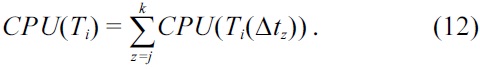
Step 8 (Calculate the cumulative probability of utilization of the current task). The algorithm balances the distribution probability, by calculating the cumulative probability of utilization (CPU) of each task to time step assignment, and then selects the tasks with the smallest CPU. The CPU of a task Ti in time step Δtij is determined as CPU(Ti(Δtij)) = DPU(Δtij) * ΔPU(Ti(Δtij)). The total CPU of a task that is scheduled from time step Δtij to Δtik is calculated as:
Step 9 (Calculate the CPU of the successor tasks). Scheduling the current task (Ti) directly affects the scheduling of the successor tasks (Tj). Hence the successor effect is also considered, while determining the total cumulative probability of utilization TCPU of a task.
Step 10 (TCPU). The TCPU of a task determines the feasibility of scheduling the task in that particular time step. The least effect determines the step in which the task has to be executed. TCPU signifies that the task graph will use fewer resources (higher utilization). The TCPU of a task Ti is given as:

Steps 7-10 are repeated for all the tasks in the task set, and a final schedule is obtained.
Step 11 (Voltage scaling). Based on the schedule developed above, voltage scaling of the tasks are performed as in the SaS algorithm, and the FCFS mapping algorithm. At every instance of the start time of a task, a check is done to see if any processor is idle. The task is scheduled on the idle processor, if any; else a new processor is initialized. The final step in this algorithm is to find the number of processors required to execute the scheduled task set. By the end of scheduling, all the tasks are ready to be executed at a specified voltage. This algorithm finally returns a schedule in which the task voltages are scaled, making sure none of the tasks miss their deadlines, and that these tasks are executed on processors in such a way that the utilization of the processors is high. The pseudocode of the PbS algorithm is shown in Algorithm 3.
Algorithm 3 Probability based Scheduling (PbS)
Inputs: A = {T1, T2, …, Tn}, PE = {PE0, PE1, …, PEm}
Outputs: σ(A), δ(Tik), α(Ti)
repeat {
determine the bound limit for tasks;
compute Probability of Utilization (PU);
compute Distributive PU (DPU);
compute Cummulative PU (CPU);
compute Total CPU (TCPU)
schedule tasks with min. TCPU;
update PU;
} until (all tasks are scheduled)
for each processor {
for each task {
scale voltages of based on slacks and deadline;
} }
} until (all tasks are scaled)
>
E. Energy-Probability based Scheduling Algorithm to Minimize Energy
The PbS algorithm proposed above reduces the concurrency of tasks in all time steps, to minimize the resources. However, the energy factor is not considered during scheduling. To achieve this, the energy-probability based scheduling (E-PbS) algorithm is proposed. The algorithm is similar to the PbS algorithm, but has an additional factor of voltage included in calculating the TCPU, called the TCPU-energy (TCPUE) factor.
Step 10 (TCPUE factor). Let V = {V1, V2, …, Vk} be the set of voltages at which a task can execute. The (TCPUE(Tik)) is calculated for different voltages Vk for the task Ti. The least TCPUE(Tik) determines the voltage at which the task will be executed. After a task is fixed in voltage, the affected distributed probabilities of utilization are updated. This process is repeated for all the tasks, and each one is scheduled for execution at a particular voltage, and the distributed probabilities of utilization are updated dynamically, to get an optimized schedule. After determining the TCPUE, the task is scheduled in the time step where the TCPU is minimal. The TCPUE of a task Ti in time step Δtj for each operating voltage Vk is determined as follows:

The value of CPU(Ti) and CPU(Tj) for the current task and its sucessor tasks are determined as shown in steps 8 and 9, respectively, in Section IV-D. The TCPUE of each task operating at a specific volatge is calculated, by multiplying a voltage factor Vr2 to the CPU terms. The voltage factor incorporates the energy awareness in the scheduling algorithm. The voltage factor Vr2 is the ratio of the current operating voltage to the maximum possible operating voltage, Vk2/Vp2. The algorithm schedules a task at a voltage in the time step where the TCPUE is minimal. Thus in this method, the voltage scaling and mapping are implicitly integrated into the scheduling algorithm. Also, initial voltages are assigned to tasks based on their respective slacks. After a task is assigned a voltage, the affected distributed probabilities of utilization are updated. This process is repeated for all the tasks, and each one is scheduled for execution at a particular voltage, and the TCPUE is updated dynamically to get an optimized schedule. The final step in this algorithm is to find the number of processors required to execute the scheduled task set, as shown in step 11 (Section IV-D). The pseudocode of the E-PbS algorithm is shown in Algorithm 4.
Algorithm 4 Energy-Probability based Scheduling (EPbS)
Inputs: A = {T1, T2, …, Tn}, PE = {PE0, PE1, …, PEm}
Outputs: σ(A), δ(Tik), α(Ti)
repeat {
determine the bound limit for tasks;
compute Probability of Utilization (PU);
compute Distributive PU (DPU);
compute Cummulative PU (CPU);
compute Total CPU-Energy (TCPUE)
schedule tasks and assign processor;
update PU;
} until (all tasks are scheduled)
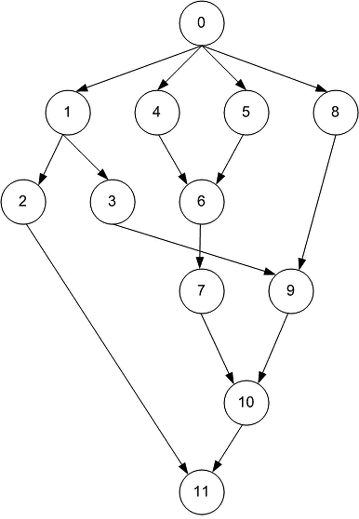
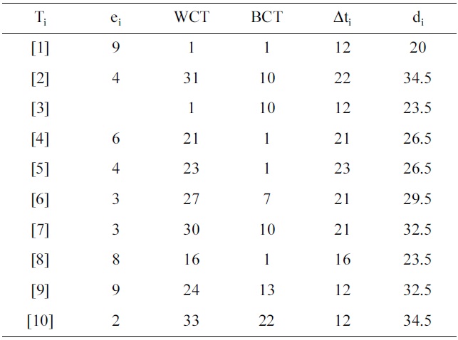
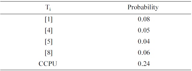
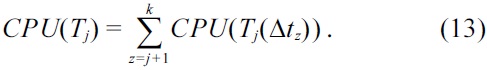
This section explains the SaS, SbS, PbS, and E-PbS algorithms, with the aid of an example. Fig. 1 shows an example task graph, consisting of ten tasks, with edges between them indicating the dependencies between the tasks. The source (task 0) and sink (task 11) tasks are redundant tasks that have zero execution time. This task graph is expressed in standard task graph (STG) format, as shown in Table 1. Only the final deadline of the end task in the STG is specified. The first step of all proposed algorithms is to determine the deadline and slack of each task, by backtracking from the sink task, as described in
Task graph example
Section IV-A. Each task Ti is represented by parameters ei, {Tj}, {Tk}, gi, hi, di, and si, which are the execution time, predecessor task set, successor task set, start time, end time, deadline and slack of the task, respectively. Also, a task executed on a processor operating at a specific voltage is simply refered to as a task operating at a specific voltage, or the voltage assigned to the task.
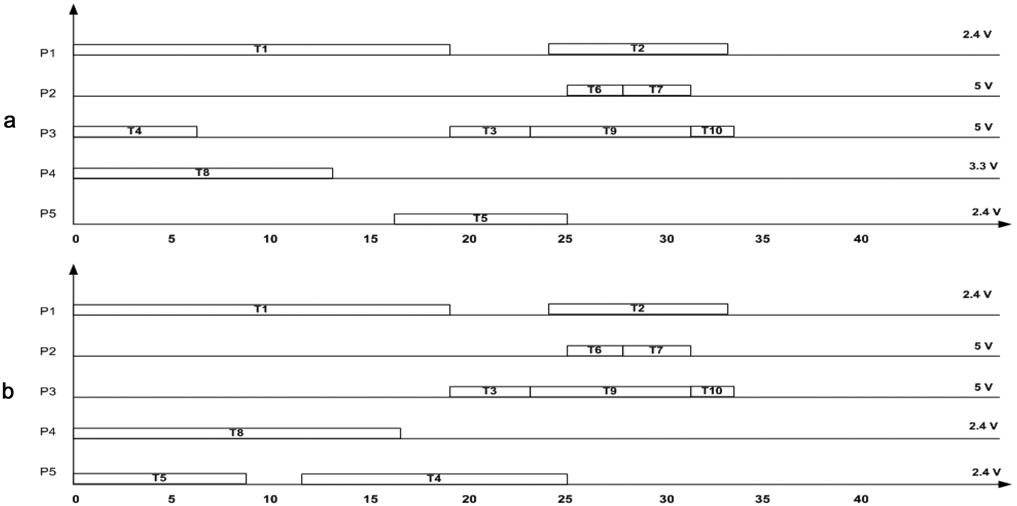
Initially, all processors are assumed to be operating at a maximum voltage in the voltage set V = {5 V, 3.3 V, 2.4 V}. The task graph and each task in the task graph meet their respective deadlines when operated at the maximum voltage. Another assumption is that each processor runs at a preset voltage, and voltage switching between tasks is not supported. In the first step, tasks with zero execution time are eliminated, and the tasks are sorted with respect to their slack. Next, voltage scaling is applied to the tasks. For the example, task T1 has the least slack (s1 = 11.5), and has an initial execution time, e1 = 9. The new execution time e1 of the task T1 at voltage 2.4 V is determined as e1 = e1×(5/2.4) = 18.75. The start and end times (? j and ? j) of all successor tasks Tk of T1, given as Tk = {T2, T3, T9, T10}, are updated with respect to the new deadline of task T1, and evaluated to see if they meet their respective deadlines. The above process is called voltage scaling. For the voltage scaled task T1, none of the successor tasks (Tk) misses its deadline, and hence the task T1 is assigned a voltage of 2.4 V. If any task misses its deadline, then task T1 is scaled to a voltage greater than 2.4 V. This process is repeated for voltages greater than 2.4 V, and checked to satisfy deadlines. This procedure is repeated for all tasks in the task graph.
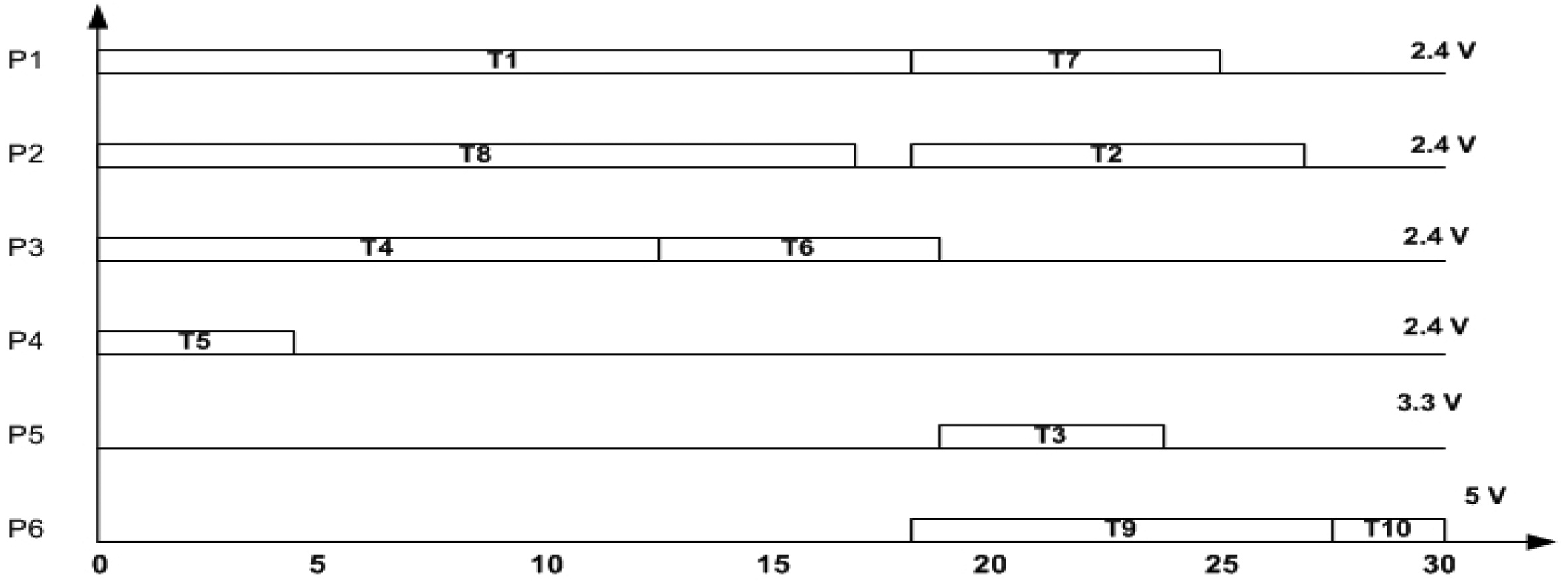
Voltage scaling of all the tasks results in partitioning the tasks into three partitions, where each partition contains tasks operating at a specified voltage. An earliest deadline first scheduling is performed on the task graphs. If a task is to be scheduled at a specific voltage and the processor operating at that specific volatge is busy, a new processor is added to the resource. The schedule developed by the SaS algorithm is shown in Fig. 2. The total number of processors required by the SaS algorithm is 6.
The SbS algorithm performs scheduling of the tasks on the available processor, before scaling the task voltages.
The algorithm proceeds by first scheduling the tasks based on the EDF scheduling algorithm. The voltage scaling succeeds scheduling by scaling each task in each processor, and determines if the following conditions are satisfied: the current task or any of its successors meet their deadlines, or any of the tasks that are executing on the same processor as the current task do not miss their deadlines. It is important to note that when a task is scaled, all the tasks on that processor are also scaled to the same voltage, because it is assumed that a processor can operate at that specified voltage. As shown in Fig. 3, the SbS algorithm starts by choosing processor P1 and task T1. The task T1 is voltage scaled to the voltage 2.4 V, and checked to see if it satisfies its deadline. If the deadline of task T1 is satisfied, the start and end times of all its successor tasks {T2, T3, T9, T10} are also modified for their start time and end time. If any task in this processor misses its deadline, task T1 is scaled to a higher voltage, and their execution times are checked, to see if all tasks satisfy their deadlines. If deadlines are satisfied, the task is operated at that voltage. This procedure is repeated on all the tasks in that processor. The total number of processors required by the EDF algorithm is 4. Fig. 3 shows the final schedule obtained using the SbS algorithm, where the processor P1 operates at 5 V, and all other processors are scaled to operate at 2.4 V.
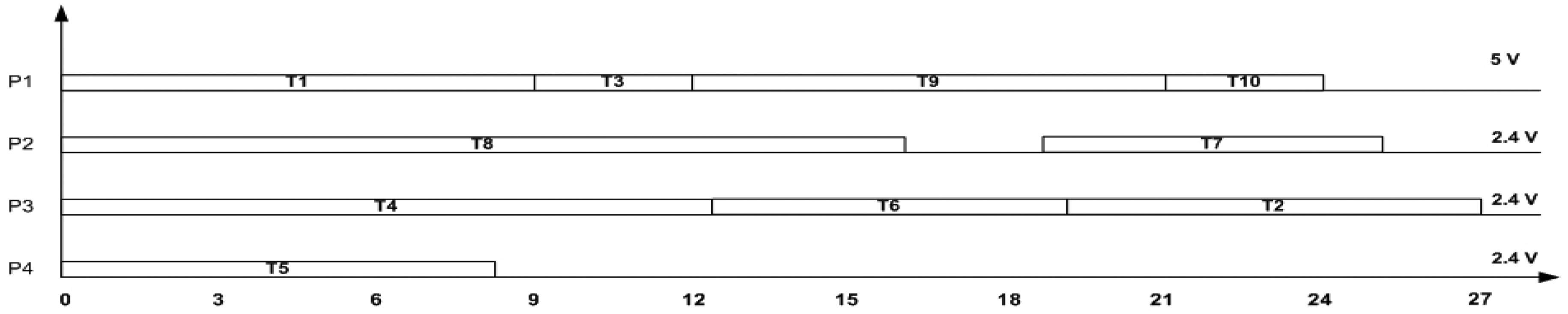
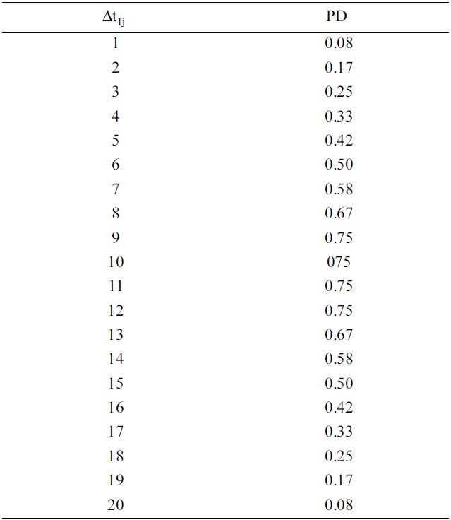
The first step in this algorithm is to determine the BCT and WCT schedules for the task graph. Since the final deadline of the task graph is ?34.5? = 34, the whole graph is divided into 34 time steps (Δtj). The bound limit for each task (Δti) is determined as shown in Equation (10). Table 2a shows the bound limit of each task, along with the BCT and WCT start times (gBCT and gWCT) of each task. For task Ti, the task has the earliest start time Δt1j = 0, and the latest start time Δt1j as 11. The next step is to determine the probabilities of utilization of each task in each time step from Δt11 to Δt111+ e1 = 20 = d1, where e1 = 9. These probabilities are determined by using Equation (11). For the example, the probabilities of utilization (PU(T1(Δtj))) for task T1 within the range Δt1j, j = 0 to 20 are given in Table 2b. After determining the probabilities of utilization of each task in each time step, the next step is to find the distributed probabilities of utilization (DPU(Δt1j)) for each time step. This is done by calculating the sum of probabilities of utilization for all task occurring in each time step. Table 2c lists the distributed probabilities of utilization for time step Δti1. Then, the CCPU(Ti) of the task is determined by scheduling the task in a control step, and finding the variation in probability of utilization, as given by Equations (12) and (13). The TCPU(Tj) is again the summation of all CPU(Ti) of a task and its successors CPU(Tj). Due to the high volume of data, the CPU(Ti) and CPU(Tk) are omitted. The task Tj that has the highest value of TCPU in time step Δt1j is scheduled in that current time step. The probabilities of utilization of subsequent time steps and tasks are updated, and the above processes repeated for sucessor tasks. Throughout this procedure, the tasks are assumed to be running at 5 V.
The next major step is to scale the voltages of the tasks in such a way that neither the task, nor its successors, miss their respective deadlines. The schedule obtained so far assumes that the tasks are assigned 5 V. Each task in this schedule is then voltage scaled, as described in the SaS algorithm. The last and final step in this algorithm is to determine the number of processors required to accommodate all the tasks in the schedule. This is accomplished as explained in step 11 of Section IV-D. The processors are assumed to be operating at only one particular voltage,
[Table 2a.] BCT and WCT start time and bound limit of each task

BCT and WCT start time and bound limit of each task
without the ability to shift voltages. The final schedule for the benchmark program 10.stg is shown in Fig. 4a.
The CPU for each task and its sucessor in time step Δti1 are evaluated as shown in step 10 of Section IV-D. The TCPUEs of a task at 5.0 V (V1), 3.3 V (V2) and 2.4 V (V3) for the task Ti are determined as shown in Equation (16), and are represented as TCPUE(TiV1), TCPU(TiV2), and TCPUE(TiV3), respectively. The voltage factor Vr2 for the above three cases is given as V12/V12, V22/V12, and V32/V12, respectively. The algorithm schedules a task at a voltage in the time step where the TCPUE is minimal. After a task is assigned a voltage, the affected distributed probabilities of utilization are updated. This process is repeated for all the tasks, and each one is scheduled for execution at a particular voltage; and the TCPUE is
[Table 2b.-1] Distribution probabilities for task T1 within the bound limit Δt1j

Distribution probabilities for task T1 within the bound limit Δt1j
[Table 2c.-2] CCPU(T1) for task T1 at time step Δti1

CCPU(T1) for task T1 at time step Δti1
updated dynamically, to get an optimized schedule. The final schedule obtained by E-PbS is shown in Fig. 4b.
Processors supporting several supply voltages are available. Various supply voltages result in different energy consumption levels for a given task Ti. The voltage at which a task is run can be decided before the execution of the task, or sometimes, when the task is executing. In the former method, a particular voltage is assigned to a task, and it is run at that voltage on the processor. In the latter case, the switching of the voltage while the tasks are running on the processor is controlled by the OS. These variable voltage processors operate at different voltage ranges, to achieve different levels of energy efficiency.
All the four scheduling algorithms have been implemented
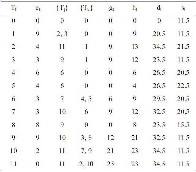
[Table 3.] Number of processors required for scheduling
Number of processors required for scheduling
in C++. The STG set were used to evaluate the performance of the above algorithms. The STG benchmark suite contains both synthetic, and practical realtime application task graphs. The assumptions followed during evaluation are as below:
All the processors operate at a pre-specified set of voltages.
All the processors operate at a constant and identical frequency.
Processors cannot shift from one voltage level to another while executing a task set. This constraint allows us to ignore overheads, such as processor voltage transition times, transition energy, states, and steps [24] during scheduling.
The switching capacitance of the processors is constant, and is the same for all the processors.
All the tasks are assumed to be non-preemptable, aperiodic, dependent tasks.
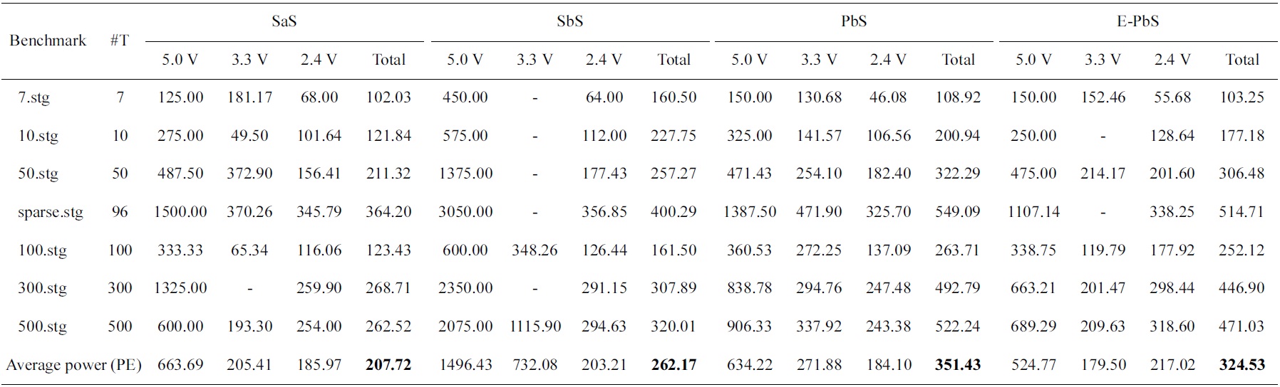
[Table 4.] Average power consumed by each processor in nWatts for the scheduling algorithms

Average power consumed by each processor in nWatts for the scheduling algorithms
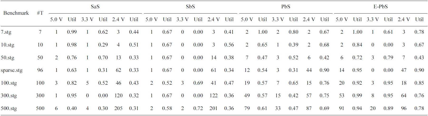
[Table 5.] Utilization of the processors for the scheduling algorithms

Utilization of the processors for the scheduling algorithms
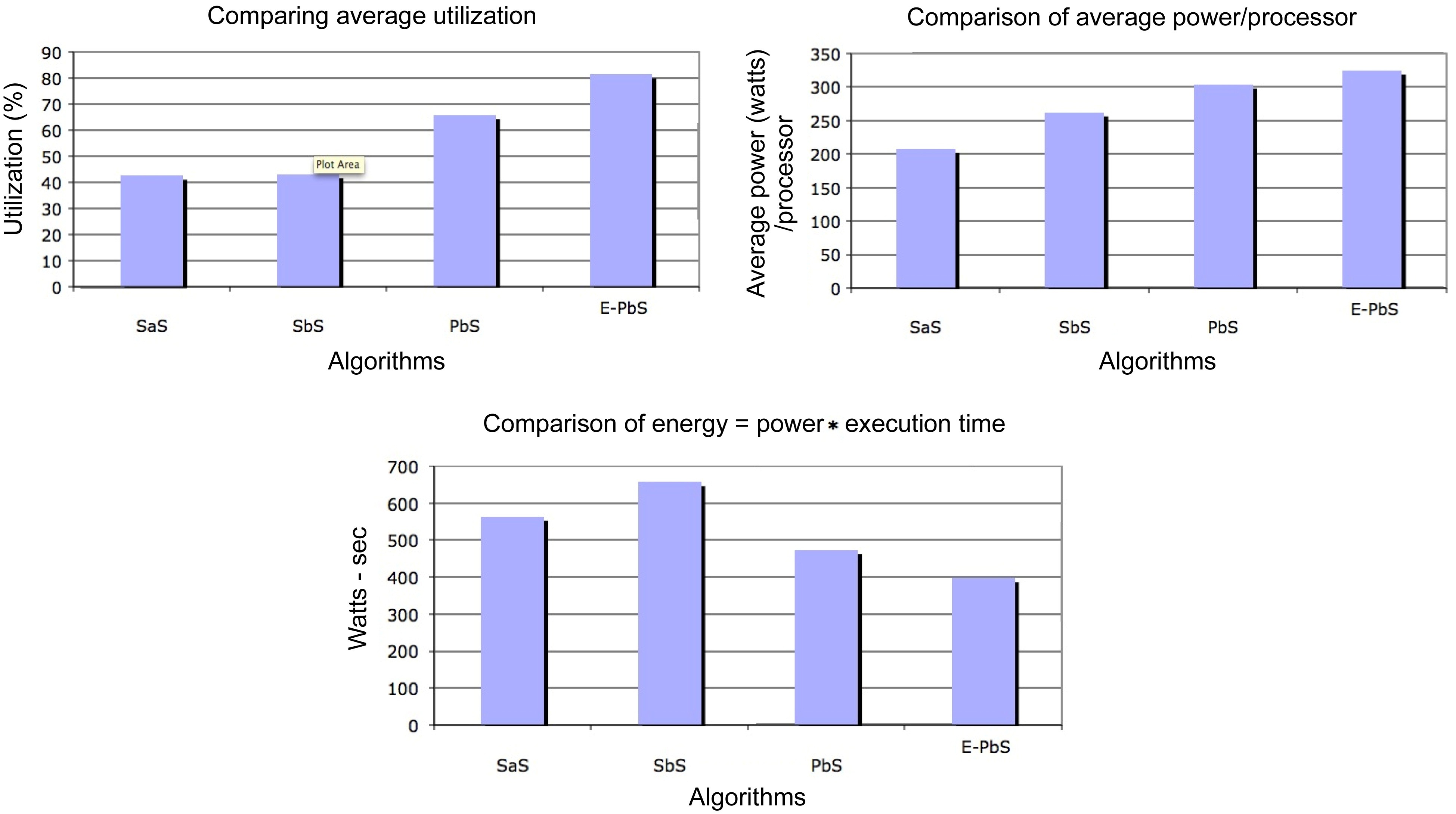
The performance of the SaS, SbS, PbS, and E-PbS is summarized below, based on the results obtained for the various benchmarks, as shown in Tables 3-5. From Table 3, we conclude that the SbS algorithm results in the smallest required processors to complete the task graphs. However, the SaS and SbS algorithms have more processors operating at 2.4 V (lowest operation voltage), and hence will have larger completeion times for the task graphs. Almost 90% of the processors operate at this voltage. On the other hand, the PbS and E-PbS algorithms have processors equally operating at all voltages (distributed almost uniformally). Table 4 shows the average processor power consumed by each algorithm (SaS = 208, SbS = 262, PbS = 351, E-PbS = 324), for each benchmark. The following conclusions are derived from Table 4: the SaS and SbS algorithms have lesser average processor power consumption (?25% less) compared to the PbS and E-PbS algorithms. Table 5 shows the processor utilization (SaS = 42%, SbS = 43%, PbS = 65%, E-PbS = 81%) achieved by the algorithms for the various benchmarks. In this case, the PbS and E-PbS algorithms outperform (?35%) the SaS and SbS algorithms. Typically, the SaS algorithm results in lower power consumption and higher completion times. This is evident by the large number of processors and tasks operating at 2.4 V (Table 3). Similarly, the SbS algorithm results in a smaller number of processors, and better completion times. The proposed PbS and EPbS algorithms results in higher processor utilizations, but with smaller completion times (Table 5). Hence, the PbS and E-PbS algorithms results in smaller energy consumption (average processor power × completion times (or utilization)), as shown in Fig. 5. In this section we provide a quick time complexity analysis of the various algoirthms implemented in this work. Let ‘
Scheduling of applications or task graphs in multiprocessor or multicore systems is an important research question that needs to be addressed, in light of today’s emerging embedded system demands. It is often necessary to develop scheduling and task mapping algorithms that optimize processor utilization and processor power consumption. This work proposes an integrated scheduling and mapping algorithm, called PbS, that optimizes the above requirements. The proposed PbS algorithm, and its variation, called E-PbS algorithm, are based on the force directed scheduling algorithm used in high-level synthesis of digital circuits. The algorithms were implemented and tested with synthetic and real application task graphs (benchmarks). The proposed algorithms are compared with traditional scheduling approaches like FCFS (SaS) and EDF (SbS). The SaS and SbS algorithms also implement an explicit mapping, or voltage scaling algorithms, after and before scheduling, respectively. The algorithms are compared for processor utilization, average power consumed per processor, and the number of processors required to implement the given set of task graphs. Based on the results discussed in Section VI, we can conclude that the PbS and E-PbS algorithms provide better processor utilization and lower energy consumption, compared to the SaS and SbS algorithms.