There are many industrial embedded systems consisting of millions of lines of code, and containing many tasks, where some tasks may have real-time constraints. Looking closer at these systems, independent tasks may consist of subtasks that exhibit strong dependencies. Subtask dependencies are necessary for realizing some control activities. That is, some subtasks have to respect a processing order due to message exchange between subtasks or usage of various resources. A significant problem in such systems is that missing deadlines can cause disastrous failures. One desirable approach to avoid timing-related errors in such complex systems is to use exact worst case response time (WCRT) analysis to provide a reliable guarantee.

Spuri [1] derived WCRT for sporadically periodic tasks (independent task instances that arrive within a certain period for a time interval, and then does not rearrive for a longer period) with arbitrary deadlines where tasks are scheduled using a preemptive earliest deadline first (EDF) scheduler. Another approach proposed by Zhang and Burns [2] obtains necessary and sufficient conditions for EDF schedulability of a set of sporadic tasks. Within a sporadic task subtasks inter-arrival time is greater than or equal to the task period. The proposed schedulability conditions reduce the calculation overhead of previous results. Zhang et al. [3] model WCRT under preemptive fixed priority, for another extension of sporadic tasks. The sporadic task model introduces a bound on the number of task arrivals allowed in a specific time window. Further, they allow a different number of task arrivals for different time windows. However, the approaches in [1-3] did not consider the precedence constraints among subtasks.

A different approach proposed in [4-7] derives WCRT analysis for a sort of sporadic task with precedence-constrained subtasks where task activation results in activation of all subtasks at the same time. That is, all subtasks arrive simultaneously as an external event occurs. To consider the precedence constraints between subtasks, the authors model a sporadic task by a directed acyclic graph (DAG). These approaches adopt a technique for transforming the DAG of the task under analysis to a simple chain by modification of the deadline of the subtasks. This technique is still somehow an approximation of the response times, because in some particular cases, transformation of a graph to a chain, and consequently introducing an artificial deadline for subtasks, is not able to exploit sufficiently the priorities among subtasks.

This paper extends the aforementioned results to a larger class of sporadic task models. Our proposed sporadic task allows an arbitrary arrival time and arbitrary deadline of subtasks with acyclic precedence constraints, i.e., within a sporadic task, subtasks include acyclic precedence constraints and arrive at arbitrary time instances with arbitrary deadlines. Subtasks are implemented upon a uniprocessor platform and are scheduled under a preemptive EDF scheduler such that subtasks with precedence constraints are scheduled according to their precedence relations, while subtasks with no precedence relations are scheduled according to the EDF algorithm. In contrast to approaches in [4-7], to acquire WCRTs precisely, no deadline modification is allowed and the analysis is performed on the original sporadic graph.

Since by adopting offset-based techniques, the corresponding analysis of a distributed system or a multiprocessor system can be transformed to an equivalent single processor analysis, our approach can be easily adopted for schedulability analysis of distributed systems or multiprocessors. In this case, task executions and message transmissions are modeled as preemptive/non-preemptive tasks executed in a single processor. In the study of schedulability of a distributed real-time system, compared with the approach proposed by Palencia and Harbour [8], our contribution is shown to have significant improved performance by a factor that grows larger with processor utilization.

This paper starts by introducing related works in Section II, and the computational model in Section III. The proposed WCRT analysis is described in Section VI. A case study is presented in Section V. Finally, our conclusions are stated in Section VI.

In the past, periodic and sporadic task scheduling has received considerable attention. A well-known result for periodic tasks is that the preemptive EDF algorithm is optimal in the sense that it will successfully generate a processor schedule for any periodic task system that can be scheduled [9]. In contrast to periodic tasks, a sporadic task is invoked at arbitrary times but with a specified minimum time interval between invocations. Kim and Naghibzadeh [10] showed the optimality of non-preemptive EDF, for the scheduling of a set of sporadic tasks with relative deadlines equal to their periods. The authors proposed the feasibility condition for a set of sporadic tasks with relative deadlines equal to their respective periods. [2] obtains the necessary and sufficient conditions for EDF schedulability of sporadic tasks, where subtasks’ inter-arrival time is greater than or equal to the task period. [3] considered WCRT for a sort of sporadic task model where a bounded number of tasks arrive in a specific time window. Spuri [1] proposed WCRT analysis of sporadically periodic task sets with arbitrary timing requirements scheduled under EDF. In this approach, sporadically periodic tasks are identified by two periods: an inner period and an outer period. The outer period is the worst-case inter-arrival time between bursts and the inner period is the worst-case inter-arrival time between task instances within a burst [1]. However, the computational model in the above-mentioned works does not cover dependency among subtasks of a sporadic task. A common form of dependency arises when one subtask produces the communication data of another consumer subtask to proceed with its computations. Further, even when no explicit data exchanges are involved, subtasks might be required to run in certain orders.

The approaches proposed by Zhao et al. [4,5], concerns WCRT analysis for a set of independent sporadic tasks, scheduled under non-preemptive EDF scheduling and with fixed priority scheduling, respectively. Each sporadic task is represented by a graph to indicate subtask dependencies. The main idea is to transform the graph to a canonical chain by modification of the deadline of subtasks appropriately so that each subtask in the obtained canonical chain has a deadline larger than its predecessors. The idea of a graph to chain transformation was inspired by the approaches proposed by Harbour et al. [6,7]. This approach uses the graph to chain transformation to provide a theoretical framework for analyzing task sets scheduled through a fixed priority preemptive scheduler. However, [4-7] cover simultaneous arrival of subtasks only.

In the study of task level precedence constraints, the meaning of a precedence constraint is applicable in practice only to tasks that have the same rate. Mangeruca et al. [11] generalizes the concept of precedence constraints between tasks to allow tasks to have different rates. Moreover, they consider integer linear problem formalization of the problems of optimum priority/ deadline assignment for preemptive EDF scheduling under precedence constraints.

As for distributed hard real-time systems, Spuri [12] adapted the Holistic analysis technique to the systems that were scheduled under the EDF.

In this work, the analysys requires global knowledge of the task routes to predict the worst-case end-to-end delay of a task. Later, [8,13-15] improved the estimations of WCRTs by developing the offset-based technique. The fundamental principle behind it is that, given the offset information of the tasks at a communication resource, the authors transform a distributed system to an equivalent uniprocessor. In this case, estimations depend only on the load that the analyzed task encounters. Another extension was proposed by Redell [16], which allows each task to have one or more immediate successors. The main problem with these techniques is that they take into account the precedence relations between tasks only indirectly, causing pessimistic resuls to quickly increase along with the system scale. In Section V, we show the outperformmance of our work compared with the work in [8].

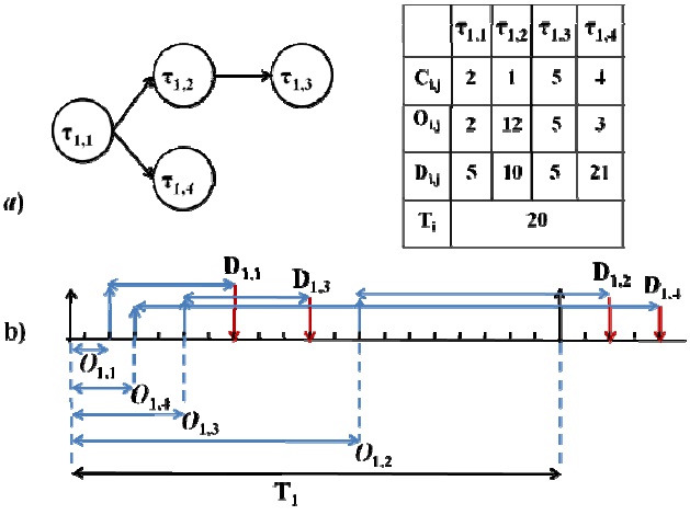
Definition. Sporadic Task (τ_i): Sporadic task τ_i consists of n_i number of preemptive subtasks τ_i = {τ_i,1, …, τ_i,ni} with precedence constraints and arbitray timing requirements. The inter-arrival time of of each task is separated by a minimum time T_i. Each task activation at time t results in activation of all subtasks, each one at time t_i,j = t + O_i,j, where O_i,j denotes the arrival time relative to the activation of the task, Fig. 1 Each subtask has an execution time C_i,j, and relative deadline D_i,j. The absolute deadline d_i,j of subtask τ_i,j requested at time t_i,j equals d_i,j = t_i,j + D_i,j. The relative deadline of task τ_i is denoted by D_i, where D_i equals D_i = max_j(O_i,j + D_i,j).

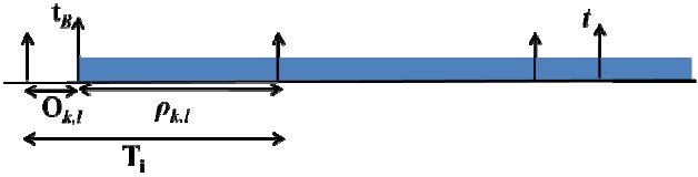
Definition. Busy Period: the time interval delimited by two successive idle times, during which the CPU is not idle. Let us denote the length of the longest busy period by L and the starting instance of the longest busy period by t_B.

Definition. Deadline-d Busy Period: A processor busy period in which only the subtasks with an absolute deadline smaller than or equal to d execute.

Definition. Worst-case Response Time (WCRT)(R_i,j): maximum possible delay between arrival time and completion time of subtask τ_i,j on each activation time of the subtask τ_i,j inside the longest busy period:

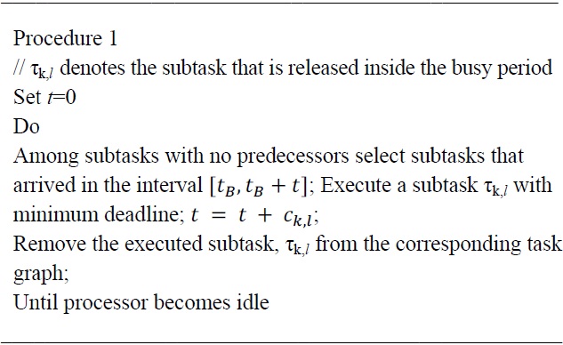
Procedure 1 determines the order of scheduling of subtasks:

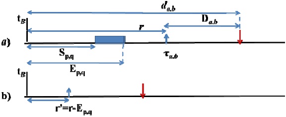
According to the generalization of an original result described by Liu and Layland [9] we simply need to study the schedule of tasks in the most demanding arrival pattern, the longest busy period. As noted in Section III, the length of the longest busy period in our model is denoted by L and the starting instance of the longest busy period by t_B. When the schedulability of periodic tasks under EDF is considered, from [17] we have: the completion time of a task’s instance with absolute deadline d, must be the end of a busy period in which all executed instances have absolute deadlines less than or equal to d (which is defined as deadline ？d busy period). If we are able to examine all such periods, by taking the maximum length we can find the WCRT of a task [17]. Let us consider the validity of the above argument for our proposed task model with precedence constrained subtasks. To do so, using a simple example illustrated in Fig. 2a, we shall demonstrate that it suffices to consider the worst-case scenario of the subtask τ_a,b with absolute deadline d that was released at r unit times after t_B, inside a deadline ？d busy period. Consider a busy period where the coincidence of some subtasks τ_p,q, with D_p,q > d occurs at t_B. Assume that the subtask τ_p,q with D_p,q > d is executed before starting instance of execution of the analyzed subtask τ_a,b, as shown in Fig. 2a. Even though τ_a,b with an earlier absolute deadline is released earlier than τ_p,q, due to the highest urgency of the predecessors of τ_a,b and their exposed precedence relations, it is possible that τ_p,q would be executed earlier. However, we show that it is possible to avoid the conservative analysis of such busy periods by introducing an equivalent deadline ？d busy period. Let us denote the phase between the starting instance of execution of the subtask τ_p,q with t_B, by S_p,q and the phase between the period can be examined that starts at arrival of those subtasks.

In this case, the subtask τ_a,b would be released at time r'=r？E _p,q, see Fig. 2b because in both of the cases, the response time of subtask τ_a,b is identical. This means that, if execution of subtask τ_p,q with D_p,q > d occurs before starting the instance of execution of analyzed subtask τ_a,b, as shown in Fig. 2a, the considered deadline ？d busy period would be finished at time t_B + S_p,q.

Thus we are interested in deadline ？d busy periods with a length greater than or equal to r.

In a scenario where the model is composed of periodic tasks (as proposed in [1]) or the task model is defined as sporadic tasks with simultaneous arrival time of subtasks (as proposed in [5]) scheduled under EDF, the worst-case busy period occurs in the synchronous busy period, where all tasks arrive simultaneously. However, since in our model each task consists of subtasks with arbitrary release times and timing requirements, we must take into account that the critical instance may not be obtained by the occurrence of all tasks at the starting instance of the busy period. Let us consider the coincidence of which subtasks of t_B would result in the critical instance. Consider subtasks of the task τ_k that possibly delay execution of τ_a,b. Each such subtask falls in the category Set_k^H, which is composed of subtasks with D_k,l ≤ d. According to the definition of the deadline ？d busy period, only the subtasks of task τ_k, k ≠ a that are included in Set_k^H are considered to delay the execution of the subtask τ_a,b by arriving inside a deadline ？d busy period. Thererore, a deadline ？d busy period could be constructed by releasing one subtask of each task with D_k,l ≤ d at t_B. However, we do not know which subtask coincident to t_B corresponds to the critical instant for the analysis of the subtask τ_a,b. Therefore, in the procedure of considering the critical instance of subtask τ_a,b, we must study all possible deadline ？d busy period created by choosing one higher priority subtask in each task to occur at time t = t_B. Fig. 3 illustrates an example showing that to construct the critical instance of τ_a,b in a deadline ？d busy period, we must consider all cases, where a higher priority subtask of each task occurs at t_B.

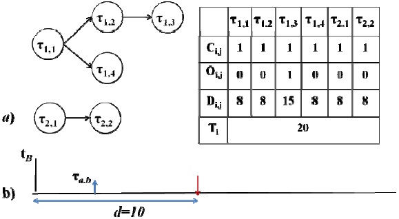
Consider a system consisting of three sporadic tasks. namely τ₁, τ₂, and τ_a. The task τ_a consists of one subtask τ_a,b with O_a,b = 4 and D_a,b = 6 where it tis released at 4 unit times after t_B, as shown in Fig. 3. The sporadic graph of tasks τ₁, τ₂ and the characteristics of corresponding subtasks are shown in Fig. 3a. The timeline of the activation time and deadline of subtask τ_a,b is shown in Fig. 3b. For simplicity, let us assume that the computation time for each subtask of every task is one unit. In this case, it is easy to show that the longest deadline ？d busy period con be obtained by releasing τ₁ and τ₂ at t_B. Hence, the response time of subtask τ_a,b equals C_1,1 + C_1,2 + C_1,4 + C_2,1 + C_2,2 + C_a,b ― 4 = 2. Let us assume another scenario defined in the same way, except that the computation time of subtask τ_1,3 equals 7. In this case, releasing the subtask τ_1,3 at t_B and releasing the task τ₂ at time t_B would lead to the longest deadline ―d busy period. Hence, the response time of subtask τ_a,b equals C_1,3 + C_2,1 + C_2,2 +C_a,b ― 4 = 6.

Theorem 1 helps us to find the worst-case scenario where τ_a,b is released at time t_B ≤ r < t_B + L:

Theorem 1: The worst-case response time of subtask τ_a,b with a release time at t_B ≤ r < t_B + L and absolute deadline d, is found in a deadline ―d busy period of subtask τ_a,b where the first activation of some subtask τ_k,l, of task τ_k, k ≠ a, with D_k,l ≤ d coincides with t = t_B and task activations of τ_k occur periodically with their maximum rate inside the busy period.

Proof: Let t₁ > t_B be the imstant at which a subtask τ_k,l, k ≠ a with absolute deadline d_k,l is activated the first time inside the busy period, and let d_k,l ≤ d. Suppose that we move t₁ to coincide with t = t_B in this circumstance; it is possible that an activation of successor subtasks of subtask τ_k,l, denoted by τ_k,j, with an absolute deadline after instant d may have been moved earlier to have a deadline before or at d; thus it would possibly increase the response time of the analyzed subtask.

Based on Theorem 1, in the procedure of finding the critical instance of subtask τ_a,b released at time t_B ≤ r < t_B + L, we must study all possible deadline ―d busy periods created by choosing one higher priority subtask in each task ot occur at time t = t_B. Given all possible deadline ―d busy periods, the largest response time of subtask τ_a,b accounts for its WCRT, denoted by R_i,j.

In the rest of this paper, the coincident subtask of task τ_k to t_B is denoted by τ_k,l. Through the analysis expressed in Eqs. (2)―(10) we shall assume that task τ_a consists of one subtask, τ_a,b, only. In the latter part of this section, we will extend the analysis to consider the response time of τ_a,b where the task τ_a includes a sporadic graph with precedence constraints.

Let us first consider a complete activation of task τ_k that occurs in the time interval [t_B, t], where t > t_B.

This activation occurs before t, so that t？'activation time' ≥ T_k and 'activation time' ？ t_B ≥ 0. We denote the total number of complete activations of task τ_k that occur in the time interval [t_B, t], by N_k,l(t). As has been noted earlier, in our analysis, we assume that the subtask τ_k,l has been released at t_B. From Fig. 4, it is easy to see that N_k,l(t) could be obtained by

where ρ_k,l represents the phase between t_B and the first activation of task τ_k inside the busy period. Hence, we have ρ_k,l = T ？ O_k,l if O_k,l > 0, and ρ_k,l = 0 otherwise. The total time required to schedule activations of task τ_k that occurred completely in the time interval [t_B, t] equals:

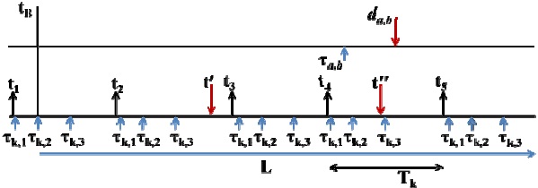
Fig. 5 represents a scenario for the alignment of the task τ_k arrival pattern after t_B. The upper part of this figure corresponds to the activation and deadline of subtask τ_a,b, and the lower part represints the activation of subtasks of task τ_k. In Fig. 4, N_k,2(t^') = 0, because t^' ？ t₂ < T_k. Further, since t^" ？ t₂ > T_k, t₂ ？ t_B > 0 and also t^" ？ t₃ > T_k, t₃ ？ t_B > 0, we have N_k,2(t^") = 2.

It should be noted that in the above discussion, we only find the time required to execute N_kl(t) activations of task τ_k. However, among those, activations of task τ_k. released after d？D_k would not contribute to the response time of analyzed subtask [17]. Thus, at each given time interval [t_B, t], only activations of task τ_k with deadlines before or at d, can contribute to the response time of analyzed subtask. At each given time interval [t_B, t], C_k,l(t) is bounded by G_k,l(d), which is given by following equation:

Therefore, the contribution of N_k,l(t) complete activations of task τ_k to the response time of the analyzed subtask, at each given time interval [t_B, t], is given by:

To see this, redoing the example in Fig. 5, let us assume that D_k,1=D_k,3=T_k, D_k,2=3？T_k-O_k,2 and hence D_k=3？T_k. In this case, we have C_k,2(t")=2.

G_k,2(d)= 0 and consequently, W_k,l(t",d)=0.

Eq. (4) only obtains the contribution of complete activations of task τ_k that occur inside the time interval [t_B, t]. The problem that remains is to obtain the contribution of activations that do not interfere with the response time of the subtask under analysis, completely.

We shall categorize those contributions of task τ_k into two sets. Set A: activations included in this set occur completely inside the time interval [t_B, t], but they have a deadline greater than d. Thus those activations do not interfere with the response time of τ_a,b, completely. For example, in Fig. 5, consider D_k,1 = D_k,3 = T_k, D_k,2 = 3 · T_k ？ O_k,2. In this case, we have W_k,2(t'', d) = 0 , but activations of task τ_k that occurred at times t₂ and t₃ consist of some subtasks that would delay the response time of τ_a,b: subtasks τ_k,1 ², τ_k,1 ³. We shall define

to obtain the total computation time of the subtasks of activations of task τ_k in Set A by

where max(E_k) represents the summation of computation time of the subtasks of activations in Set A that have an absolute deadline less than or equal to d and activation time before or at t, so that all their predecessors also have an absolute deadline less than or equal to d and activation time before or at t. In Fig. 5, consider D_k,1 = D_k,3 = T_k, D_k,2 = 3 · T_k ？ O_k,2, we have

Set B: activations included in this set do not occur completely inside the time interval [t_B, t]. This set may consist of two members only. The first one is the first activation that occurs immediately before t_B, where O_k,l ≠ 0 , for example, activation of task τ_k occurred at time t₁ , in Fig. 5. The second member of Set B is the last activation, where t？′activation time′ < T_k. Consider time interval [t_B, t′] in Fig. 5: activation of task τ_k occurs at time t₂ and corresponds to this element. We shall define

to account for the total computation time of the subtasks of activations of task τ_k in Set B by:

where max(E_k) is defined as for Eq. (5). Finally, we shall define δ_k,l(t,d) to obtain the total computation time of the subtasks of activations of task τ_k in Set A and Set B by

So far, we have studied the contribution of task τ_k to the response time of τ_a,b that has been released until time t. In general, the study of response time of a subtask τ_a,b with deadline d is an iterative procedure. The basic idea is that in each step, the obtained busy period must be the end of the execution of all instances of all tasks with deadlines less than or equal to d that have been released in the previous steps. Toward this, we shall define LN_a,b(t,d)^(k) to represent the length of the resulting busy period in the k^’th iteration of response time analysis of subtask τ_a,b with deadline d, where t is substituted with the length of the obtained busy period in the previous step. LN_a,b(t,d)^(k) is ob-tained by the iterative equation, Eq. (9). This equation represents the iterative procedure, where at each step the length of a busy period is given by the summation of execution times obtained in Eqs. (4) and (7). We shall initiate this iterative procedure by Eq. (8). In Eq. (8), c_k,l represents the execution time of the subtask coincident to t_B. The iteration is halted where the computations converge.

The response time of subtask τ_a,b where it occurs at time t_B ≤ r < t_B + L is

The problem that remains to be solved is to determine the response time of subtask τ_a,b, where task τ_a includes a sporadic graph with precedence constraints. Consider a scenario where τ_a,b is released at r. In this case, the response time of τ_a,b is influenced by the order of execution of all subtasks of task τ_a that must be scheduled before τ_a,b. Further, this sequence of subtasks of task τ_a may not be the same as the sequence of subtasks in another scenario where τ_a,b is released at r′. Therefore, it is of great importance to determine the order of subtasks of task τ_a that must be scheduled before τ_a,b for each release time of τ_a,b.

In order to find the correct response time of subtask τ_a,b, we shall use Procedure 1 to determine the correct sequence of subtasks of task τ_a that must be scheduled before τ_a,b. This procedure would let us to consider the correct sequence of subtasks of task τ_a that must be scheduled before τ_a,b and consequently the correct response time of subtask τ_a,b. To show this, let us denote the current subtask of task τ_a of which its response time has been considered by τ_a,q and the next chosen subtask by τ_a,p. Consider a scenario where τ_a,b is released at r. In this case, τ_a,q and all the subtasks of task τ_a that have been considered by Eqs. (8) or (9) will be dropped from the sporadic graph of task τ_a, by Procedure 1. When τ_a,p is chosen as the analyzed subtask by Procedure 1, it must have the minimum deadline among all subtasks of task τ_a that arrived at or before the completion of execution of τ_a,q, but they have no predecessors. This fact is in accordance with the definition of scheduling mentioned in Section III.

We have compared the results of our proposed analysis, with the results obtained by Palencia and Harbour [8]. This approach transforms a distributed system schedulability analysis to an equivalent analyzable uniprocessor schedulability test, by using task offsets. Since tasks are preemptive, without loss of generality, we applied the static offset technique on a set of chains of subtasks, where each node in a chain represents a preemptive subtask.

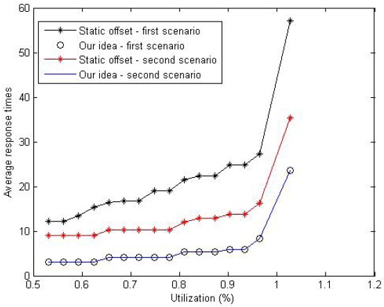
Fig. 6 shows the obtained average response time by our analysis and obtained average response time by the static offset technique proposed in [8]. We ran our simulation on a task set consisting of 20 tasks, each one including five subtasks. The average response time corresponded to five subtasks of an analyzed task. The x-axis represents the processor utilization which varies with the changing execution time of the subtasks in the task set. The deadline of subtasks in the task set is generated randomly, except the 2nd subtask of each task in the first scenario and 2nd and 4th subtask in the second scenario. In the first scenario, the deadline of the 2nd subtask of each of the 20 tasks is generated so that it is greater than the deadline of the analyzed task. In the second scenario, the deadline of the 2nd and 4th subtask of each of the 20 tasks is generated so that it is greater than the deadline of the analyzed task. For the first scenario, it can be seen that the average response time obtained by the static offset technique is between 3 to 5 times larger than that of our results. The reason is that the static offset technique accounts for the execution time of the 3rd, 4th, and 5th subtasks of the interfering tasks in the task set where they do not contribute to the response time of the analyzed subtasks. In fact, it accounts for the execution time of each interfering subtask assuming that the corresponding predecessors have a deadline less than the analyzed subtask. This is a result that is shown to be flawed by [7] in the case of fixed priority scheduling. As for the second scenario, it can be seen that the difference between the average response times is tighter. However, our simulation same results as the first scenario. The obtained smaller average response times by the static offset method is due to accounting for the execution time of the 3rd and 5th subtasks of the interfering tasks in the task set. However, in our constructed scenario, since the task offsets are set to zero, by the definition of the deadline busy period, they do not contribute to the response time of the analyzed subtasks.

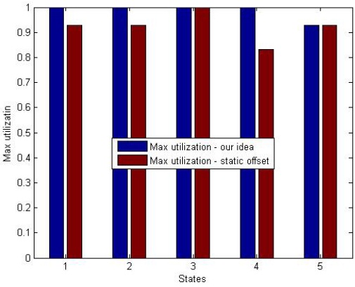
In order to evaluate the pessimism of the admission controllers of our analysis and the static offset-based method implemented on a uniprocessor, we conducted simulations to identify the lowest utilization at which deadlines are missed. We perform our simulation on a set of 30 tasks with 5 subtasks per task, in one processor, for the case in which the task offsets are zero. Task sets were generated randomly, and the subtask specifications do not represent worst-case scenarios. We add a new task, denoted by τ_a, with 5 subtasks with randomly generated deadlines, accordingly. We increased the utilization of the task set by increasing the execution time of subtasks uniformly, until deadline misses were observed. Fig. 7 presents the results of our analysis where the y-axis represents the utilization and x-axis represents 5 states. Under state 1 (2, 3, 4, 5) each task has the first (and second, third, fourth, and fifth, respectively) subtask in its corresponding chain with a deadline greater than D_a. Each bar in Fig. 7 presents the results from the simulations of the lowest utilization at which the deadline misses were observed for different task states in the system.

It can be observed that for our analyzed task model, the new task τ_a can be admitted for all utilizations in the first 4 states. In the 5th state, τ_a can be admitted for utilizations below 90%. In addition, for the first 4 states, the maximum utilization of the task set at which τ_a can be admitted, by the static offset based method, fluctuates between 80% in the 4th state and 100% in the 3rd state. As previously mentioned, the drawback of the static offset-based analysis is that it accounts for the execution time of each interfering subtask assuming that the corresponding predecessors have a deadline less than D_a. The 2nd, 3rd, and 4th state can be similarly described, indeed. However, in the 5th state, both methods have the same results.

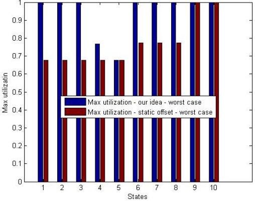
In another experiment, we consider a scenario where the task sets represent the worst-case scenario. In this case, all the subtasks with a deadline less than or equal to D_a have a deadline less than or equal to the minimum deadline of the subtasks of task τ_a. Fig. 8 presents the results of our analysis where the Y axis represents the utilization and x-axis represents 10 states. The first 5 states are tested as explained for Fig. 7. State 6 represents a scenario where the 1st and 3rd subtask have a deadline strictly greater than D_a. State 7 represents a scenario where the 1st and 4th subtask have a deadline strictly greater than D_a. State 8 represents a scenario where the 2nd and 4th subtask have a deadline strictly greater than D_a in state 9 and 10, subtasks 1st, 4th and 5th and 2nd, 4th and 5th, respectively, have a deadline strictly greater than D_a. In this case, due to the drawback pointed out for the last experiments, it can be seen that the maximum task set utilization obtained by the offset based technique degrades significantly.

In this paper, we studied the exact WCRT analysis of sporadic tasks that are modeled by DAG and scheduled under preemptive EDF scheduling. The objective is to obtain precise WCRTs of a generalized sporadic task model with arbitrary timing requirements that have not been considered in previous works. A nice feature of our work is that it exploits the precedence constraints between subtasks in an accurate way while taking advantage of the deadlines of subtasks. We find via simulation results that our methodology provides accurate results comparable with existing works.