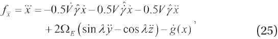
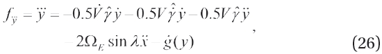
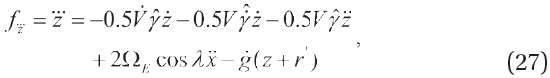
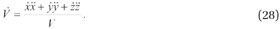
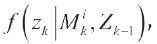
This paper studies the problem of tracking a re-entry vehicle (RV) in order to predict its impact point on the ground. Re-entry target dynamics combined with super-high speed has a complex non-linearity due to ballistic coefficient variations. However, it is difficult to construct a database for the ballistic coefficient of a unknown vehicle for a wide range of variations, thus the reliability of target tracking performance cannot be guaranteed if accurate ballistic coefficient estimation is not achieved. Various techniques for ballistic coefficient estimation have been previously proposed, but limitations exist for the estimation of non-linear parts accurately without obtaining prior information. In this paper we propose the ballistic coefficient β model-based interacting multiple model-extended Kalman filter (β-IMM-EKF) for precise tracking of an RV. To evaluate the performance, other ballistic coefficient model based filters, which are gamma augmented filter, gamma bootstrapped filter were compared and assessed with the proposed β-IMM-EKF for precise tracking of an RV.
This study considers the tracking and impact point prediction (IPP) of a re-entry space launch vehicle with unknown ballistic coefficients and air densities. The tracking of a re-entry vehicle (RV) (Costa 1994, Bar-Shalom et al. 2001, Farina et al. 2002) is an extremely important problem for safety assurance through a correct ground IPP. In the case of a space launch vehicle, the major objective is to transport and place satellites into orbit. Thus it is designed to be launched in accordance with an elaborate predetermined trajectory. Thus far, however, quite many cases of launch failures have occurred. If an abnormal thrust halt or an abrupt departure from a planned path happens, it is necessary to track the vehicle or predict the impact point in real time for safety concerns. As for a scenario of a true target trajectory, we assumed that the vehicle has launched normally with beacon mode tracking, but an abnormal situation occurs 170 seconds after lift-off. The vehicle’s thrust is terminated and no communication is available with ground stations. At that time the beacon mode tracking function is halted and the mode should be adjusted as not to lose the target.
Tracking an RV and its IPP are the subjects to estimate the state variables of the dynamic model of a ballistic target. The performance of an estimation filter depends on the target dynamic model, the measurement model, and the filter structure. The uncertainties normally found during target modeling are ballistic coefficients, mass of target, initial values of state variables, and aerodynamic reference area, etc. From among these, the estimation of the ballistic coefficient is crucial for precise tracking of an RV. These subjects have been studied vigorously over the past decades. Mehra (1971) performed a comparison of an RV’s tracking performance using non-linear filters including the extended Kalman filter (EKF). Siouris et al. (1997) proposed the extended interval Kalman filter for the precise tracking of an RV. Cardillo et al. (1999) introduced a new tracking filter using EKF for re-entry objects with uncertain drag. Also, Minvielle (2005) reviewed the RV tracking chronology and introduced several non-linear filters including EKF. According to previous research, various tracking algorithms using EKF were proposed by linearizing the non-linear system to estimate the ballistic coefficients as well as other kinetic states, such as position, velocity, and acceleration. Typically the constant ballistic coefficient (CBC) filter was introduced to estimate the ballistic coefficient β (Dwivedi et al. 2005), the constant drag parameter (CDP) filter to estimate the drag parameter α, which is defined as the inverse of β (Mehra 1971), and the gamma augmented (GA) filter to estimate the gamma (γ) which is defined as the function of β and air density ρ (Bar-Shalom et al. 2001). Recently, Ghosh & Mukhopadhyay (2011) proposed the gamma bootstrapped (GB) filter which estimates basic kinetic states in the main filter with bootstrapping the separately estimated γ and its derivative from the sub filter. If the target modeling is inaccurate in a single model filter, especially for maneuvering target tracking, an estimation error may increase or diverge. To overcome this disadvantage of a single model filter, Blom & Bar-Shalom (1988) introduced the interacting multiple model (IMM) filter algorithm. The IMM filter is known for superior performance in tracking maneuvering targets and has high applicability in a variety of fields. For tracking a ballistic target, Farina et al. (2002) proposed a 4-model IMM filter which consists of a 6-dimensional Kalman filter (KF), a 9-dimensional KF, and 2 different CBC model KFs, and Farrell (2008) proposed a 3-model IMM filter which had a constant axial force model, a ballistic acceleration model, and standard auto-correlated acceleration Singer model. Particularly, Yuan et al. (2010) made use of an IMM filter to estimate the thrusting state for the purpose of IPP.
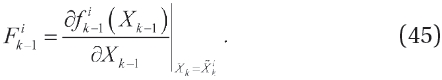
In this paper, we propose the ballistic coefficient β model based IMM-EKF (
2. THE REFERENCE FRAME AND THE TARGET MODEL
2.1 The Reference Frames for the Motion of an RV
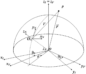
The motion model of an RV is assumed to be a point mass which is applied to the rotating ellipsoidal earth. The difference between the actual and dynamic model is modeled as process noise. The reference frames used for an RV’s dynamic model are the Earth-centered-inertial coordinate system (ECI-CS), the Earth-centered-earth-fixed coordinate system (ECEF-CS) and the East-north-up coordinate system (ENU-CS) (Regan 1984, Siouris et al. 1997, Li & Jilkov 2001).
In Fig. 1, ECI-CS, OxIyIzI, is a fixed inertial frame as its origin is the center of the earth. It is a right-handed system with the origin O. Here the axis OxI points to the direction of the line where the longitude crossing the launch point of the vehicle and the equator meet. The axis OzI points to the direction of the North Pole. ECEF-CS, OxFyFzF, which has a rotational motion with the earth as its origin, is on the same position with ECI-CS. The radar ENU-CS, OxNyNzN, which has the origin ON, is fixed on the surface of the earth where the tracking radar is placed. The up direction of ENU-CS, ONzN, is normal to the earth’s surface whereas ONxN axis points east and ONyN axis points north.
Dynamic models (Li & Jilkov 2001, Ghosh & Mukhopadhyay 2011) are used to estimate the tracking of an RV. The issues of the ballistic and re-entry phase can be analyzed with respect to gravity and drag only. We derive the acceleration model of an RV.
2.2.1 Gravity
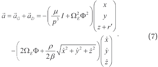
The acceleration of RV by gravitational force (Regan 1984, Bar-Shalom et al. 2001) in the ECI-CS can be expressed as:
In Eq. (1), μ is a universal gravitational constant as μ=3.986006 × 10¹⁴ m3/sec2 and p is the position vector of an RV. Eq. (1) can be expressed in the ENU-CS as:
whereas

is the angular velocity vector of the earth’s rotation,

is the Coriolis force and
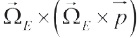
is the centrifugal force. From Eqs. (1) and (2), the gravitational acceleration in the ENU-CS is
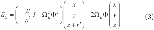
whereas Ф is the coordinate transformation matrix and r' is the distance between the radar and the center of the earth.
2.2.2 Drag
The acceleration by drag force is as:
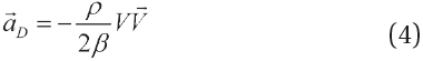
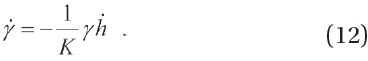
whereas the ballistic coefficient (Regan 1984, Dodin et el. 2005) is defined as:
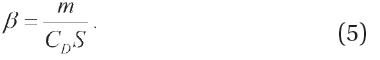
Note that m denotes the mass, CD denotes the aerodynamic drag coefficient and S denotes the cross-sectional reference area of the RV. β is basically an unknown parameter to be estimated during the tracking of an unknown RV, but if all information of an RV is known, it is quite possible to directly calculate β. In Eq. (4) the air density ρ can be modeled as a function of altitude h as follows:
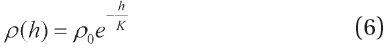
whereas the parameters ρ0 and K of the target are given as in Table 1, based on the 1976 US standard atmosphere model
[Table 1.] Air density model parameters.

Air density model parameters.
(United States Committee on Extension to the Standard Atmosphere 1976) . Eq. (6) is used to generate the true target trajectory.
2.2.3 The Acceleration Model of an RV
From Eqs. (1) through (4), the acceleration model of RV in re-entry phase is as:
3. BALLISTIC COEFFICIENT BASED ALGORITHMS
In this section, we introduce several ballistic coefficient model-based estimation algorithms which are evaluated as distinguished tracking performances in previous papers. These are the GA filter and the GB filter. In addition, we designed the
3.1 Measurement Model for the Filters
A measurement model is designed and used commonly in filter algorithms. Measurements which are modeled in the radar ENU-CS are the relative range, elevation, and azimuth between the target and the tracking radar. The measurement equation is as:

whereas:
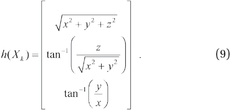
In Eq. (8) the measurement noise vector
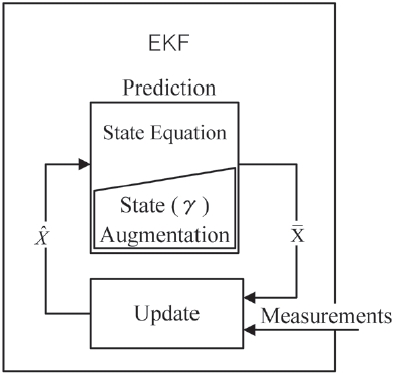
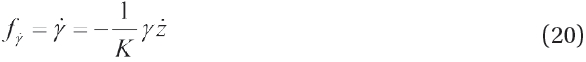
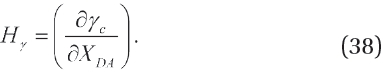
The GA filter is a type of ballistic coefficient based estimation algorithm, but it regards the variation of air density additionally which significantly affects the nonlinearity of the system. Thus the GA filter estimates γ, which is composed of the ballistic coefficient β and the air density ρ, while a ballistic coefficient augmented filter (Mehra 1971, Dwivedi et al. 2005) does only β. The basic idea of the GA filter is that the new state γ is simply augmented in the state equation as described in Fig. 2. The other procedures are the same as EKF (Grewal & Andrews 2001).
3.2.1 Gamma Model
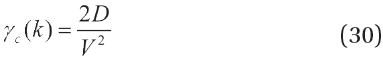
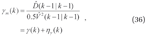
The ballistic coefficient β is a function of the aerodynamic drag coefficient as shown in Eq. (5). Also, the air density model ρ in Eq. (6) may vary according to the altitude of the target. Thus β and ρ can be estimated and calculated using intricate numerical formulae (Regan 1984). A parameter γ can thus be defined as:
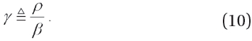
Here, ρ is modeled by the relation as in Eq. (6) and β is approximated by a linear function model of the altitude h (Bar-Shalom et al. 2001) as follows:

Through combining Eqs. (6, 10, 11) and taking the first derivative of γ, we obtain:
3.2.2 State Equations of the GA Filter
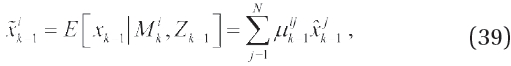
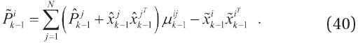
The state equation of the GA filter is as:
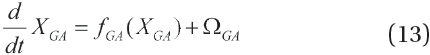
whereas,


Furthermore,


where

was obtained from Eq. (12).
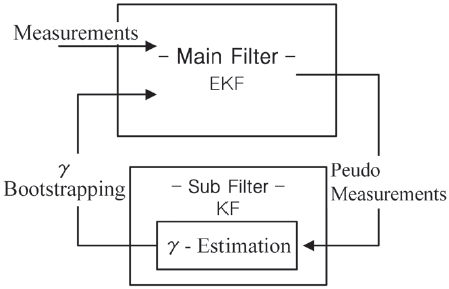
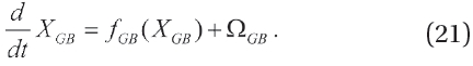
The GB filter by acceleration and jerk models was proposed in (Ghosh & Mukhopadhyay 2011). The GB filter handles ballistic coefficient β through gamma estimation similarly to the GA filter, but it uses a particular method of bootstrapping. To implement such bootstrapping, the GB filter is divided into two parts, being a main filter and sub-filter as described in Fig. 3.
The main filter is used to estimate the kinematic information including target position, velocity and acceleration while the sub-filter estimates

The estimated results from the separated sub-filter are then bootstrapped into the main filter. Ghosh & Mukhopadhyay (2011) introduced two models of acceleration and jerk for the GB filter and presented that the GB filter had better tracking performance than the GA filter. However, the jerk model may adversely affect the estimates of other
parameters, such as position, velocity, acceleration and jerk, if the rate of change of jerk is not estimated accurately. Thus, we adopt only the acceleration model filter to compare its performance with the other filters.
3.3.1 GB Main Filter State Equations
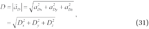
The GB main filter estimates the target position, velocity, and acceleration by modeling and integrating jerk terms. The gravity, drag and Coriolis force are taken into account in the model states. The state equation of the main filter is as follows:
Hereas:


Furthermore:
Here,

which are estimated in the sub-filter are bootstrapped into the main filter and
position. We used the EKF for non-linear estimation. The linearized state transition matrix, Ф
whereas the updated value of

at time k is used.
3.3.2 GB Sub Filter
3.3.2.1 Measurement Equations of Sub Filter
At the prediction step, the states

are predicted in the sub filter and are expressed as
At the update step, the states in the sub-filter are updated by the pseudo measurements
is used at the prediction step in the main filter. The following equations describe the pseudo measurements
whereas:


3.3.2.2 State Equations of Sub Filter
Assuming that
is a constant with additive white Gaussian noise, we can adopt the KF algorithm. Thus the GB sub-filter can be derived through a constant velocity model as a quadratic form:
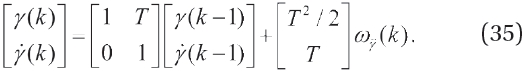
The state variables are updated using the pseudo measurements as in Eq. (30).
whereas
Whereas:
3.4 The Ballistic Coefficient Model Based IMM Filter
The IMM filter (Blom & Bar-Shalom 1988), which combines probabilistically the estimated variables from multiple dynamic models is well known as an algorithm that has similar computation load with the generalized Pseudo Bayesian approach of the first order (GPB1) (Bar-Shalom et al. 2001) and has estimation accuracy with the generalized Pseudo Bayesian approach of the second order (GPB2) (Bar-Shalom et al. 2001). In this section, we introduce the IMM-EKF algorithm and derive the state equations of
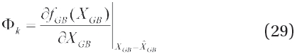
3.4.1 The IMM-EKF Algorithm
A distinct feature of the IMM filter algorithm is the combination process where the estimated mean and covariance are produced through the computation of mode probabilities. Mode probability means the probability where each filter dynamic model matches the target dynamic model. The process noises

which mean the uncertainties of a dynamic model, are white Gaussian noises with a zero mean and a covariance of

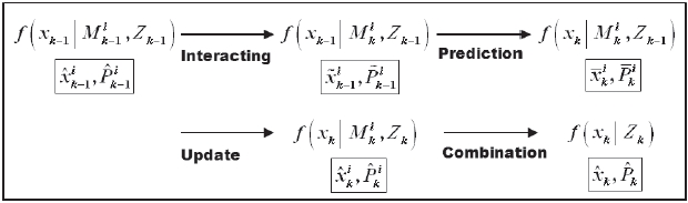
The IMM filter algorithm is composed of the steps of interaction, prediction, update, and combination which are derived under Bayes’ rule. The flow of probability density of each step is represented in the following Fig. 4.
3.4.1.1 Interaction
At the interaction step as in Fig. 4 the estimated mean
and error covariance are obtained by the conditional probability density function (CPDF),
which is computed using the transition probabilities of each hypothesis as in the following:
Here, the mode probability

and the state transition probability
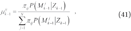
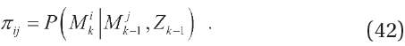
3.4.1.2 Prediction
At the prediction step as in Fig. 4, the predicted state and error covariance of
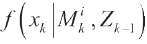
is calculated as the manner of EKF:

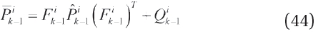
whereas:
Here

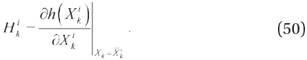
is the Jacobian matrix that uses partial derivatives of the non-linear function in Eq. (57) with respect to X.
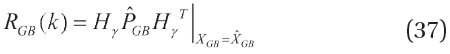
3.4.1.3 Update
At the update step in Fig. 4, the estimate and error covariance of
are calculated as EKF:


whereas:


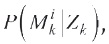
Mode probability

which means the probability of the hypothesis

is true, can be calculated as follows:
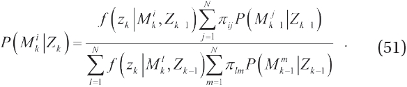
Here the likelihood function,
is calculated using measuring residual
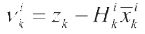
and innovation covariance

as follows through the condition of linear Gaussian.
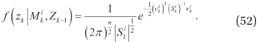
Here, n is chosen as 3 for the dimension of the system.
3.4.1.4 Combination
At the combination step, one combined estimate and error covariance are computed with the estimates

the error covariance

and the each mode probabilities
which are obtained from the multiple modes according to the Gaussian mixture model as follows:
3.4.2 The Ballistic Coefficient Model based IMM-EKF
In this paper we propose the
whereas:


Hereas:


Here, i means the i-th hypothesis of the i-th mode target dynamic model. Each model has different ballistic coefficients in different modes. Thus the β term in Eqs. (59) through (61) for
3.4.3 Modeling of β
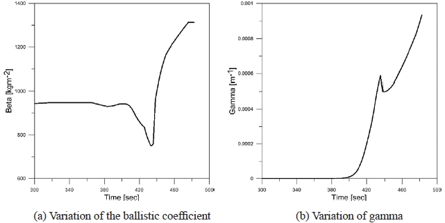
The tracking performance of
Fig. 5 shows the true β and γ of the nominal trajectory. In Fig. 5a the range of true β value is about 750-1,320 kg/m2, which were acquired by computer simulations during
[Table 2.] Design of ballistic coefficients.
Design of ballistic coefficients.
the flight range from 300 seconds to 482 seconds. Fig. 5b shows the gamma variation through the computation of (10) with the corresponding β. In this paper, the performance comparison of
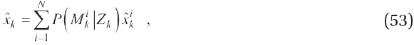
In Table 2, we selected three hypotheses or modes since the variation of the β value in Fig. 5a is not very wide from the minimum to maximum values, and since the computation time can be shortened by small numbers of β models. Thus we designed three ballistic coefficient models with the values of 800, 1,200, and 1,600 kg/m2 respectively for the three hypotheses based on the range of true β as in Fig. 5a.
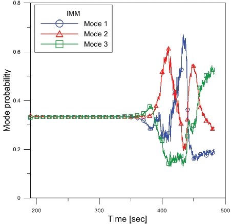
Fig. 6 shows the change of mode probabilities at each mode after tracking simulation for the true RV model. Since observability is not built, three modes have the same averaged values until approximately 350 seconds of flight time. Considering the entire flight during the re-entry phase, the mode probabilities begin to actively change after about 350 seconds when observability is formed. Thus, after about 350 seconds, each mode has its own variations of probability according to the flight conditions which are related with Eq. (5).
From approximately 380 to 420 seconds, the probability of Mode 2 rises to about 0.6 while that of Mode 1 and 3 have
0.25 and 0.15 each. From 420 to 440 seconds, the probability of Mode 1 rises to about 0.7. After about 450 seconds, the probability of Mode 3 rises to about 0.5 until the RV impacts the surface of the earth.
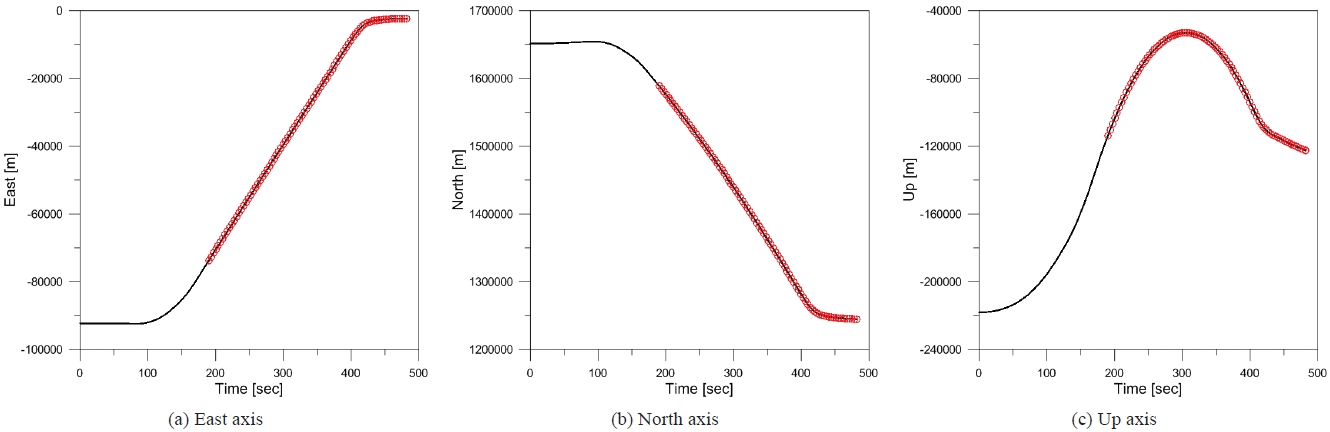
For the true trajectory of an RV, the specifications of a small low earth orbit satellite launch vehicle, the Korea SLV-I (KSLV-I), was used in the computer simulation. The true target trajectory assumes that the vehicle is safely launched at first. The predetermined thrust duration is 230 seconds but the thrust is assumed to be cut off due to an abnormal condition at Lift-off +170 seconds. Then the RV enters the coast phase. For simple analysis, the conditions of body tumbling or splitting of the RV are not considered. The launch point is set at longitude 126 degrees east and latitude 34 degrees north. The launch direction is 170 degrees from the North Pole. The results are 482 seconds of total flight time, 427 km of down range, and 113 km at the highest altitude for the nominal trajectory. The radar station for tracking is located at longitude 127 degrees east, latitude 19 degrees north. The skin mode tracking begins at Lift-off 190 seconds when the relative distance between target and radar is about 1,594 km. The tracking filter receives measurements from the sensor at a 16 Hz cycle in the form of range, elevation, and azimuth (r,θ,ψ) in polar coordinates. The measurement noise is white Gaussian with standard deviation (25 m, 0.05 deg, 0.05 deg). Figs. 7a-c represents the true target trajectory with respect to the East, North, and Up axes, respectively. The trajectory was generated in the
radar ENU-CS after proper coordinate transformations were performed from the ENU-CS referenced at the launch point. The entire trajectory is represented by the solid black line, and the tracking interval is expressed by the scattered red circles on the trajectory.
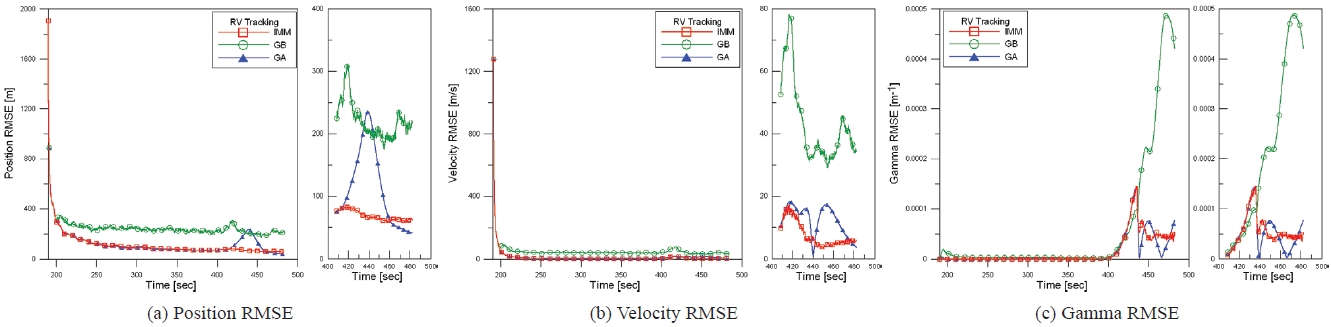
4.2 Comparison of Root Mean Square Error
Fig. 8 shows the estimation root mean square error (RMSE) in terms of position, velocity and γ for each algorithm. In Figs. 8a and b, the position and velocity of RMSE, both the
[Table 3.] Comparison of run time per scan.
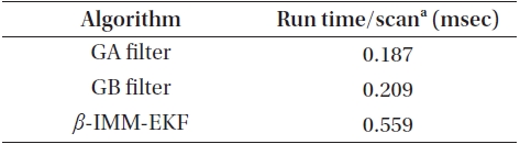
Comparison of run time per scan.
Table 3 shows the processing time per scan for each algorithm based on our simulation environments. As for the run time speed per one scan, the GA filter proved to be the fastest. This result can be expected regarding the dimensions of each filter. As described, the state equations in Sections 3.2-3.4, the dimension of the GA filter is 7 whereas that of the GB filter is 9 and that of the
The run time results represent that it seems to be approximately proportional to the dimensions. That is, the GA filter is somewhat faster than that of the GB filter, but rather had similar results since the difference is only 2 dimensions between the two. The run time results of the
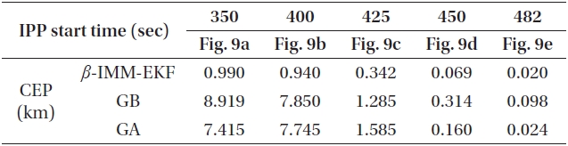
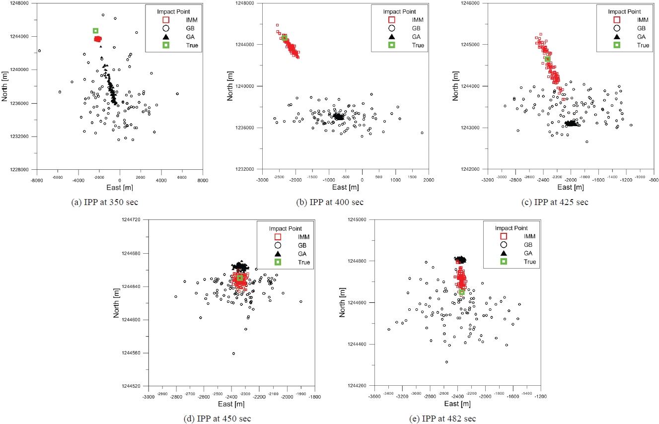
The comparisons of IPP are conducted at 5 points. These are the points at 350 and 400 seconds where drag has a small effect due to light air density; and the points at 425 and 450 seconds where drag has a significant effect at less than approximately 35 km altitude. Only the prediction step for each filter is performed without measurements. Lastly, the impact point is shown through full tracking from 190 to 482 seconds.
Fig. 9 shows the results of the predicted impact points obtained from each starting time by performing 100 Monte Carlo runs for each algorithm. In Figs. 9a and b, both the

Comparison of CEP.
GA and GB filter show an error radius up to about 15 km around the true impact point while the
Table 4 shows the values of circular error probable (CEP) based on the results of the IPPs for the three algorithms. The CEPs are computed by mean square error between the true impact point (TIP) and the predicted impact point (PIP) of the target. Each value represents the maximum radius from TIP as the center of the circle where the 50% of PIPs are located. In all cases, we can find that the
A comparative assessment of tracking performance and IPP of an RV has been performed for the GA filter, GB filter, and the proposed
Concerning the RMSE of position, velocity and gamma, the
equivalent performance during certain sections. However, some unstable oscillations appeared in the GA filter while no oscillations in occurred in the
Concerning the IPP,
Concerning the algorithm execution time per scan, the GA filter was the fastest whereas the
In conclusion, the proposed