As the benefits of formation flying using the small satellites were on the rise, a variety of researches on determination of precise relative position have been conducted. For example, there are PRISMA Mission (D’Amico 2012) launched in 2010 to test the determination of precise relative position and control that can be used in the subsequent formation flying mission, and SWARM Mission (Friis-Christensen 2006) scheduled to be launched in 2013 as a formation flying mission using the three satellites to measure the Earth's magnetic field. Both missions are based on the global positioning system (GPS). The existing researches using the GPS are largely divided into sectors of post-processing and real-time orbit determination. In researches on orbit determination for post-processing, it is known that the determination with centimeter-level precision can be made in determination of absolute position (Roh et al. 2009). In researches on real-time orbit determination, it is known that the determination with meter-level precision can be made in determination of absolute position while the determination with millimeter-level precision can be made in determination of relative position (Shim et al. 2009, Park el al. 2009, 2010). However, the GPS-based determination of relative position for satellite cannot be applied to the orbit unable to receive the GPS data. In addition, even when the inter-satellite distance is short, there is a precision level limit in determination of relative position by the nature of data provided. On the other hand, because the inter-satellite laser has the advantages that it is suitable for mounting on a small spacecraft and makes the estimation of real-time relative position available in every orbit, there have been made the researches on its use for proximity operations like rendezvous or docking, etc. Wang et al. (2011) have performed the determination of real-time relative position using the laser radar within a distance of 1 km. In this study, Hill’s equation not containing the perturbation was used for equation of motion, and the centimeter-level results in real-time determination of relative position were obtained using the laser radar with centimeter-level observation errors.
Unlike other exiting researches using the laser, in this paper we used as relative state vectors, the differentiated absolute state vectors after numerically integrating the equation of absolute motion of each satellite including the non-linear perturbation for determination of high-precision relative position even at a long distance. Based on the equation of motion including the perturbation and precise measurement of distance with sub-micrometer level observation errors, we intend to determine a more precise relative position compared to existing researches. If the high-precision relative position can be determined on a real-time basis even at a distance more than 1 km, the space-based interferometer telescope can be realized through maintenance of precise formation based on that positioning. The results may be applicable for scientific missions like a variety of missions under research in exoplanet exploration program for the purpose of finding the extraterrestrial planets (Lawson 2011).
The system using the inter-satellite laser has the advantage that the determination of relative position can be made not relying on GPS as well as the advantage that it is a precise system applicable at a long distance.
Karlgaard (2006) has performed the determination and control of relative position using the inter-satellite laser radar in low lunar orbit. However, in that research, the linearized equations of motion was used and the perturbation was not included. In this study, we integrate the state vectors of chief satellite and deputy satellite respectively using the equation of absolute motion including the perturbation in order to use an equation of precise motion. We assume that the state vector of chief satellite is obtained through the GPS in that process. However, because it is possible to determine the relative position through dynamic equation and observation of relative state vectors even when the GPS information is not received for long hours, the research for the purpose of using inter-satellite ranging in maintenance of formation flying is in progress (Xu et al. 2012). In consideration of this case, we performed the determination of relative position using a system based on the laser when the GPS information was not received for long hours.
In this section, we describe the preliminary study in preference to determination of relative position using the laser simulator. Based on extended Kalman filter (EKF) which is a real-time estimation algorithm, we implemented the algorithm to determine the relative position using the Hill’s equation which is an equation of relative motion and Gaussian observation errors. Through this preliminary study, we will investigate how the precision level in determination of relative position differs depending on Q, R matrices which are the tuning parameter of the EKF.
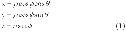
Because the system using the inter-satellite laser receives as observation values, the distance, azimuth and elevation angle which are the spherical parameters, it is easy to use the dynamic equation expressed as the spherical parameters for constitution of measurement model (Wang et al. 2011). In addition, because Hill’s equation is the linearized equation with respect to a chief satellite, having the advantage that it is easy for analyzing the relative motion, we used it as the dynamic equation for preliminary study. Using the relationship between rectangular coordinate and spherical coordinate like Eq. (1), Hill’s equation in terms of spherical parameters is expressed as Eq. (2) which is used as dynamic equation. Hill’s equation is expressed through parameters, x, y, z, which represent the values of radial, in-track, cross-track of chief satellite, respectively. ρ,θ and ? refer to the relative distance, azimuth, and elevation angle, respectively from chief satellite to deputy satellite, and ω indicates angular velocity.
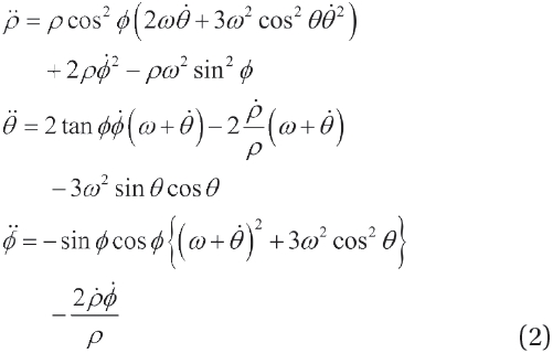
The summarized sequence to determine the relative position is as follows. First, the calculated relative state vectors are obtained by orbit propagation of initial relative state through dynamic equation, Eq. (2). Next, the observation values are created by adding the Gaussian errors to true state vectors. Finally, the state vectors are estimated through filtering algorithm. For this, we used the
[Table 1.] Measurement noise and filtering error.

Measurement noise and filtering error.
EKF as an estimation theory, and the EKF algorithm is the same as shown in the following Eq. (3) (Zarchan & Musoff 2005).
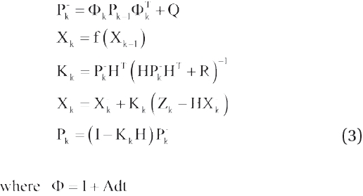
where P indicates a covariance matrix, Q indicates a process noise matrix, H indicates an measurement model, R indicates an measurement noise matrix, respectively in the state vector. The magnitude of Gaussian error which is used to create observational values is that of measurement noise, R matrix. Q and R matrices are assumed as diagonal matrix. K indicates Kalman gains, and Z indicates the observation values. A is Jacobian matrix of the equation of relative motion, and can be obtained every step numerically. The inferior letter, k means the step, and the superior letter, ? means the calculated values prior to observation renewal. Because the observation values are spherical parameters, the measurement model H is represented as [I3×3 03×3] (Wang et al. 2011).
In the EKF, it is important to determine the magnitude of process noise and measurement noise, since the determination of position is performed as placing a weight to the lesser of noise magnitude. Assuming that the dynamic equation is recognized correctly, we performed the simulation for R larger than Q. The observation error, R is set arbitrarily to see the changes in determination of relative position according to noise magnitude. The magnitude of fixed process noise, Q was obtained empirically, and the value is diag [1e-6 m 1e-9 rad 1e-9 rad 1e-8 m/s 1e-11 rad/s 1e-11 rad/s]. The simulation was performed for two cases in which the precision level of observation value is not the
same each other. The chief satellite revolves round a circular orbit with radius of 7,000 km, and the chief and deputy satellites form a projected-circular orbit with radius of 10 km. This setting is applicable to a long-distance rendezvous process at a low orbit. The results of simulation and examples are summarized in Table 1. Table 1 represents the values of R and results in determination of relative position in two examples.
In both cases explained in Table 1, the magnitude of parameters of Q corresponding to relative state vector is smaller than R, which means the dynamic model is more reliable than observation values. Therefore, it is possible to determine the relative position with precision values smaller thantude of observation errors, and we can confirm that the more precise relative position was determined compared to observation values both in Figs. 1 and 2. In case thattude of Q is smaller than that of R, the errors in determination of relative position are always less than observation errors, so the more precise relative position was determined in Example 2 in which the observation errors were relatively less than those in Example 1.
In Example 2, the parameters of Q and R corresponding to distance are of the same magnitude, and in case of the parameters of Q and R corresponding to angle, the magnitude of Q is 100 times smaller than that of R. We can confirm that in case of distance, the determination similar to observation was performed, but in case of angle, the determination about 10 times more precise than observation was performed. Through these results, we could see the importance of precise dynamic equation, and changes in results of determination of relative position depending on tuning of Q and R.
Hill’s equation has the disadvantages that in case of long distance between satellites, the errors become larger, and that it is difficult to implement the dynamic model including perturbations. For the purpose of overcoming these disadvantages, and in order to implement to conditions similar to actual outer space environment, we used the method to obtain the inter-satellite relative position and relative velocity by integrating the two-body equation including the perturbation numerically. The perturbation acting mainly to low earth orbit (LEO) satellite was added as shown in the following Eq. (4).
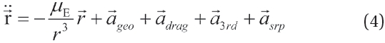
where μE indicates standard gravitational parameter of the Earth,

indicates position vector of the satellite,
refer to perturbation by non-spherical property of the Earth, resistance due to air, gravitation of the Sun and the Moon, acceleration of perturbation due to solar radiation pressure, respectively. By integrating the Eq. (4) numerically, the state vector is obtained in Earth-centered inertial frame (ECI) for each satellite. The ECI was defined as J2000. The JGM3 model, spherical harmonic 70 x 70 degree, was used for perturbation by non-spherical property of the Earth, and the exponential model was used for perturbation by air. For the perturbation due to gravitation of the Sun and the Moon, and solar radiation pressure, we referred to Vallado & McClain (2007). The orbit of satellite set in this study is a LEO with about 700 km altitude, where the perturbation acting on satellite dominantly is the perturbation by non-spherical property of the Earth, which acts with acceleration 100 to 10,000 times greater than that of other perturbation cases. So, as for geo-potential model, we used a more precise model than other perturbations.
The equation of relative motion including perturbation can be represented in spherical parameters through numerical method. The relative state vectors are differences in state vectors in the ECI coordinate system between two satellites (Leung & Montenbruck 2005). The relative state vectors represented in the ECI coordinate system are converted into the RSW coordinate system (also known as Local-Vertical Local-Hrizontal frame) which is the reference frame of chief satellite. R axis is in the direction of the position vector from the center of Earth toward the chief satellite, S axis is collinear with the velocity vector aligned with local horizontal, and W axis is normal to orbit plane. Each axis can be calculated numerically every time step (Vallado & McClain 2007).
The relative position in RSW frame can be represented in spherical parameters as shown in Eq. (5) using the definition of Eq. (1) as follows. The dynamic equation,
In this study, the laser-based observation values are used. It is assumed that the relative distance between satellites among spherical parameters determining the relative position are observed using the laser, and the angles of deputy satellite based on the chief satellite,
i.e. azimuth and elevation angle corresponding to laser direction are obtained through attitude determination of chief satellite.
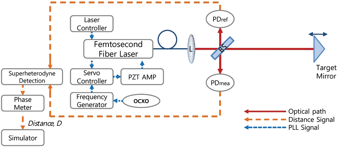
As laser algorithm to obtain the relative distance among observation values, we used the principle of synthetic wavelength interferometry among diverse methods for distance measurement using the laser. The synthetic wavelength interferometer is a method for distance measurement based on the principle that various synthetic wavelengths corresponding to from minimum several tens of millimeters to maximum several meters are created through beating among frequency modes of optical comb of femtosecond laser and thereafter are used for distance measurement (Kim et al. 2005). The femtosecond laser used in this study enables us to obtain the precision level in measurement of sub-micrometer level at several hundred kilometers range owing to its characteristic of very narrow pulse width of femtosecond laser, and a constant interval among pulses retroactive to frequency standards, which is required by next generation space projects based on formation flying. Fig. 3 is the conceptual design for equipment to measure the relative distance between satellites. In Fig. 3, a photo detector to detect the reference signal is indicated as PDref,etector to detect the signal from target mirror for measurement is indicated as PDmea, a lens for collimation of femtosecond laser is indicated as L, a beam splitter is indicated as BS, an amplifier to supply the power to piezoelectric transducer (PZT) is indicated as PZT AMP, and a crystal clock to provide the stabilized frequencies is indicated as OCXO.
The actual distance up to measurement target can be calculated by measuring the phase differences between reference signal detector and measurement signal detector, and in general, when measuring the distance shorter than long wavelength, it can be measured at once without determining the integer number of ambiguity separately. However, for the distance of several hundred kilometers, it is necessary to determine the integer number of ambiguity, and for this, two similar long wavelengths are used. The process to measure the relative distance between satellites at a long distance is largely divided into the phase that overcomes the ambiguity using two similar long synthetic wavelengths, and the phase that obtains high-resolution distance using the short synthetic wavelength (Doloca et al. 2010). First, two phase measurements are obtained using two long synthetic wavelengths as shown in the following Eq. (6).
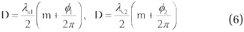
where D indicates measurement distance, λs1, λs2 refer to the first and the second long synthetic wavelengths, respectively, and m indicates integer ambiguity, ?1, ?2 indicate phase value measured by the first and the second long synthetic wavelengths. D has the same value because the same target was measured. So, writing down these two equations in terms of integer ambiguity m, the results are made into Eq. (7).
where two long synthetic wavelengths, λs1, λs2 are known values, and two phases, ?1, ?2 are measured values, so m can be calculated. When the integer ambiguity, m is determined, this value is substituted into Eq. (6), and thereafter our desired distance measurement, D can be calculated. Then, with short synthetic wavelength, high-resolution distance can be measured from the same process. In this paper, we used two long wavelengths with 10 m and 9.9998 m, respectively and short wavelength with 0.01 m obtained through RF beating among frequency modes of optical comb of femtosecond laser with 1,550 nm wavelength. The reason why we use the wavelength with 1,550 nm is that commercial optical elements are developed mostly in this wavelength area showing the least loss in optical fiber. In addition, because in light-interception, the bore of optical system vs. wavelength is large compared to wavelength of visible ray area, it has the increased effect of light-interception efficiency more than several hundred times, which contributes to reducing the bore of optical system in the actual outer space, being connected to weight reduction.
We assumed that the azimuth and elevation angle corresponding to angles in a laser-based observation were obtained through the attitude of chief satellite. Assuming that the inter-satellite laser alignment to obtain the laser signal was made exactly, only the information on distance is received after the signal acquisition is performed, so in order to know the direction of deputy satellite in the RSW coordinate system, we should know the attitude of chief satellite. Therefore, we can say that in the angle information on laser direction, there are the uncertainty as much as the errors in determination of attitude of chief satellite, and its magnitude is about 1e-5 rad (Lam & Crassidis 2007). The algorithm to determine the attitude is not included in this study, and as angular observation values, we use the true value plus the Gaussian errors having the standard deviation of 1e-5 rad which is the magnitude of errors in attitude determination of chief satellite.
We used the EKF in order to determine the real-time relative position between satellites using a non-linear equation of motion. The EKF is a real-time estimation technique which renews the observation values after obtaining the calculated values through a dynamic model.
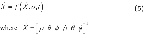
The dynamic model and measurement model that we used are shown in Eq. (8).
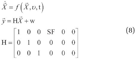
where
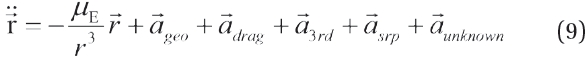
The EKF algorithm that we used is shown in Eq. (3). Assuming that there is unknown perturbation in the equation of absolute motion, Eq. (2) for numerical simulation, we used it as true value for reference. The equation of motion to which a small value of acceleration is added can be implemented as shown in Eq. (9), and the magnitude of

was assumed as 1e-14 m/s2.
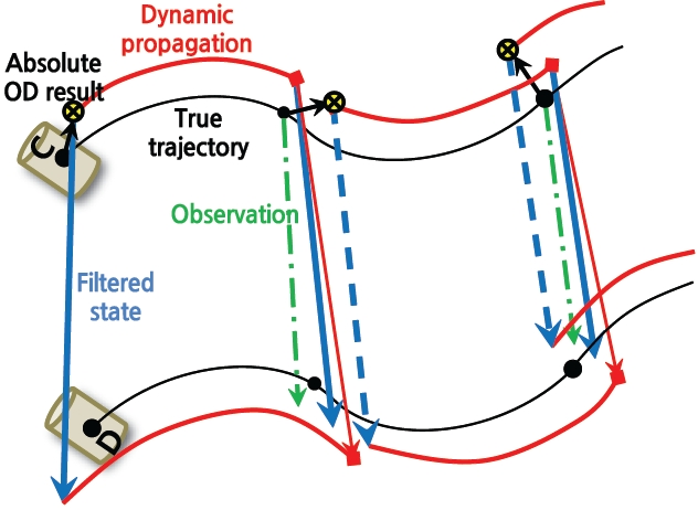
The algorithm to determine the relative position based on the EKF is as follows. It is assumed that through determination of absolute position using the GPS, we can know the state vectors of chief satellite among state vectors of each satellite required for orbit propagation in filtering process. It can be obtained by adding to true values the Gaussian errors of 1 m level (Shim et al. 2009) known as the errors in determination of absolute position using the GPS. It was assumed that the determination of orbit for chief satellite was performed every 30 seconds based on the GPS data, and the determination of relative position is performed every 1 second. During the time that the determination of orbit for chief satellite is performed through the GPS data, the state vectors of chief satellite are obtained through orbit propagation. The state vectors of deputy satellite are obtained by adding the filtering results of relative position to determined state vectors of chief satellite, and the orbit propagation for each satellite is performed in the ECI coordinate system. When the calculated relative state vectors are corrected by observation values in accordance with the EKF algorithm, the inter-satellite relative position can be determined. The concept of determining the relative position is shown in Fig. 5.
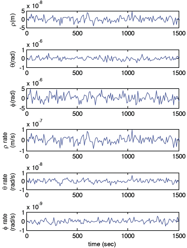
Fig. 6 shows the errors of relative state vectors due to errors (distance 1 m, velocity 1 cm/s) in orbit determination of chief satellite after orbit propagation with 1 second step size in case that the distance between two satellites is 10 km. In view of characteristic of algorithm that the state vectors of deputy satellite are obtained after the state position is added to state vectors of chief satellite, and thereafter the orbit propagation is performed for each of them, we can know that the orbit propagation of relative motion is affected by errors in determination of orbit for chief satellite. The standard deviation for each error is represented as 1.6e-8 m, 1.8e-7 rad, 1.9e-6 rad, 3.1e-8 m/s, 2.1e-9 rad/s and1.9e- 10 rad/s, respectively. These errors affect the uncertainty of
dynamic model in filtering algorithm for determining the relative position.
We performed a simulation using the aforesaid dynamic
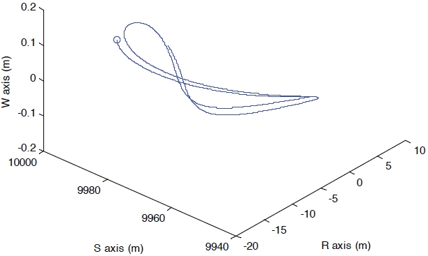
equation, observation values, and filtering process. We arranged the orbit of deputy satellite to be shaped as a leader-follower in a circular orbit with altitude of 685 km, orbit inclination angle of 98.13 degree by referring to the orbit of KOMPSAT-1 revolving the Sun synchronous orbit. On the Sun synchronous orbit, satellite can observe a specific point regularly, so the advantages of observation or communication with a ground station may follow. A variety of missions like NIMBUS, TIROS, COBE, CALIPSO, etc., having the Sun synchronous orbit have already been performed. Since the dynamic equation including the perturbation experienced by low orbit satellites is used, we intended to promote the easiness of analysis by setting a leader-follower which can be arranged simply. The initial relative distance between two satellites is about 10 km, and the distance is subject to change due to perturbation. Since
we used the dynamic equation including perturbation, we can confirm that the relative position in RSW coordinate system is changed as shown in Fig. 7.
The initial covariance matrix of relative state vector, P is the square of initial standard deviation SIG, which is the matrix with diag [1e-3 m 1e-5 rad 1e-5 rad 1e-5 m/s 1e-7 rad/s 1e-7 rad/s]. The magnitude of measurement noise used in the EKF algorithm is set in consideration of laser simulator performance and errors in attitude determination, and we obtained the values to improve the performance empirically for magnitude of process noise. In case that the relative distance is 10 km, the magnitude of w which is the standard deviation of measurement noise is represented as diag [1e-7 m 1e-5 rad 1e-5 rad], and R is the square of w. The magnitude of v which is the standard deviation of process noise found empirically is diag [1e-5 m 1e-8 rad 1e-8 rad 1e-7 m/s 1e-10 rad/s 1e-10 rad/s], and Q is the square of ν. The integrator used in orbit propagation is Runge-Kutta 7-8th order, and performs the integration at the fixed-step of 1second level.
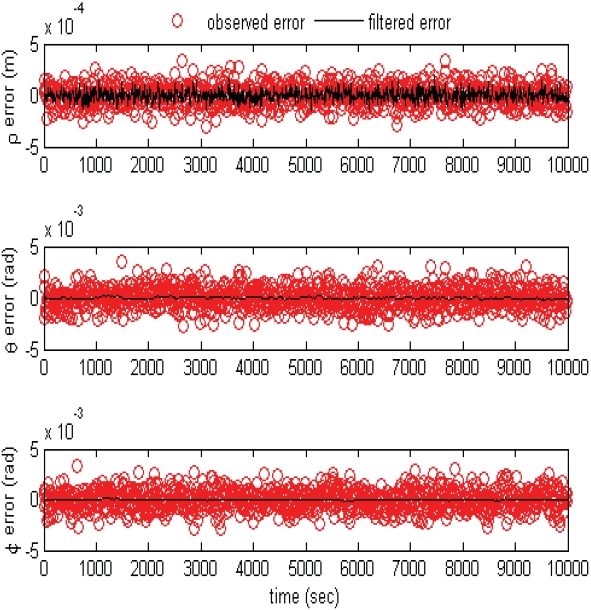
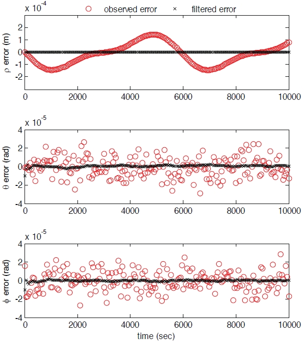
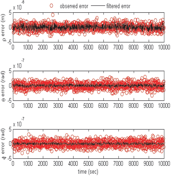
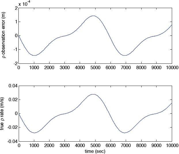
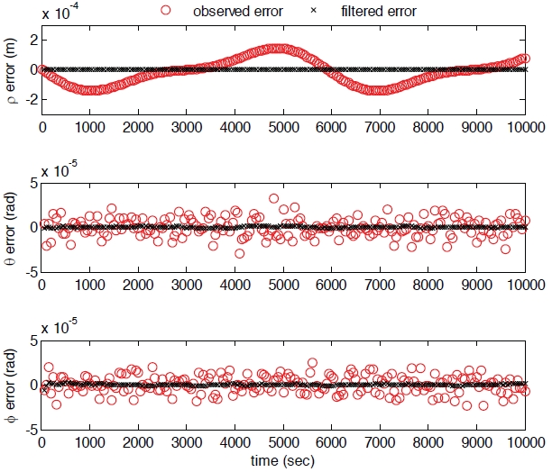
Under these conditions, the results of determination of relative position are shown in Fig. 8. In case of relative distance, we can confirm that the drift seen in observation values was removed through filtering. When the drift is removed, the uncertainty of dynamic model becomes greater than that of observation, so, the precise estimation values can be obtained by placing a weight to observation
values. In case of angle, the uncertainty of dynamic model is smaller than that of observation. Therefore, we can confirm that as a result of filtering, the magnitude of estimation errors is smaller than that of observation errors.
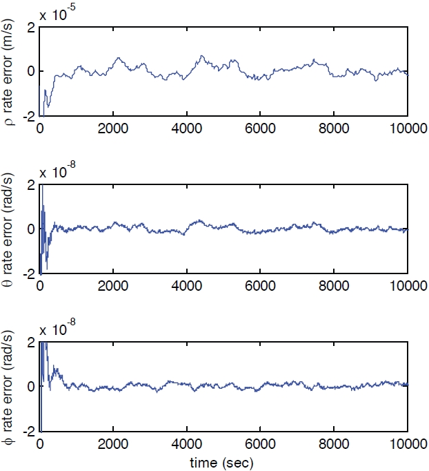
Fig. 9 represents the estimation errors for rate of change of distance, azimuth and elevation. The values for rate are obtained by equation of motion since the information for rate is not observed. In particular, the estimation values for rate of change of distance are used for removal of drift in distance observation.
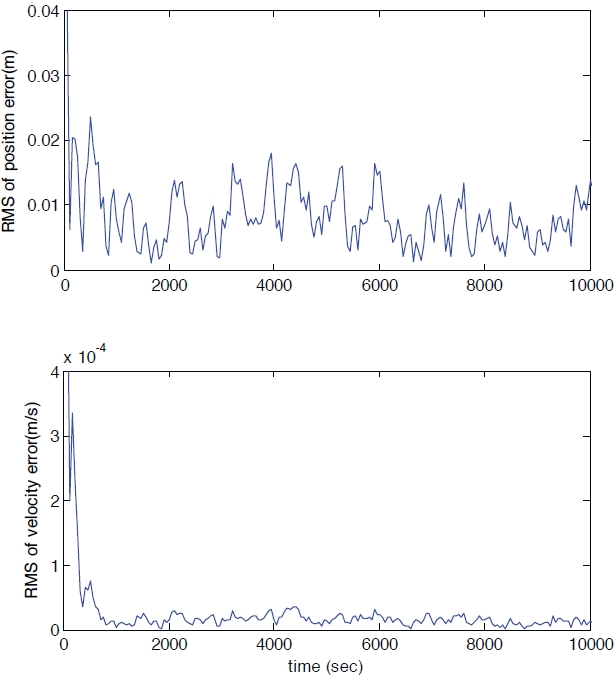
Transforming the estimation results obtained by spherical parameters to RSW rectangular coordinate system, the magnitude of errors in determination of relative position can be obtained in three-dimensional sense. Because the errors in determination of absolute position for chief satellite were included in filtering algorithm, the true values and estimation values are represented in different RSW frame, respectively. The differences between true values and estimation values represented in each RSW frame are shown in Fig. 10. The above figure shows the values of root mean square (RMS) for errors of relative position in three-
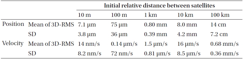
[Table 2.] Accuracy of relative position determination varying with distance.

Accuracy of relative position determination varying with distance.
dimensional space, and the below figure shows the RMS values for errors of relative velocity in three-dimensional space.
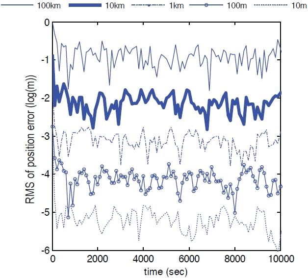
Assuming that the stabilized relative position is determined from after about 500 seconds, the average of stabilized errors is represented as 8.0 mm, 16 μm /s, respectively. Because in case of angular errors, the farther the distance between satellites becomes, the greater the errors in three-dimensional space becomes, it is possible to perform a more precise position as the distance is near. Because the precision level is expected to become lower as the distance becomes far, we made an attempt to perform the determination of relative position additionally for a variety of distances.
Fig. 11 shows the changes of precision level in determination of relative position depending on changes of inter-satellite distance. The precision level in determination of relative position after 500 seconds have elapsed is shown in Table 2.
In the vicinity of 100 km which is the limit to be measured precisely by femtosecond synthetic wavelength laser developed until now, it is possible to determine the relative position at 10 cm level, and in the vicinity of 1km, it is possible to determine the relative position showing the sub-millimeter level errors which are more precise than the results that GPS is used. Within the proximity operational scope of 100 m, it was

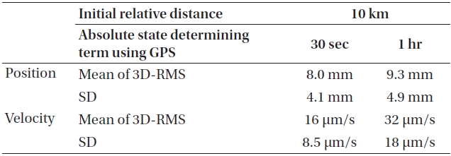
Accuracy of relative position determination varying with absolute state determining term using GPS.
possible to determine the relative position with precision level of several ten micrometers.
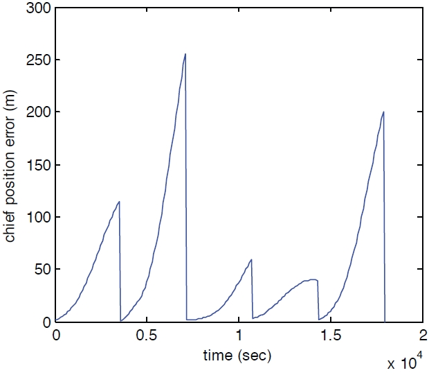
Next, in order to confirm the impact of determination of orbit for chief satellite on determination of relative position, we performed a simulation for the case that the GPS data was not received for long hours. An independent determination of relative position in determining the position of chief satellite is not possible for the system because for implementation of precise dynamic model, the state vectors of deputy satellite are obtained after adding the filtering results to state vectors of chief satellite, and thereafter the orbit propagation for each satellite is performed. However, even when the GPS data is not received for long hours, it is possible to determine the relative position based on dynamic model and laser system. We assumed that the determination was performed through renewal of the GPS observation once in 1 hour, and during the interval time, we used only the values obtained through orbit propagation based on dynamic model as state vectors of chief satellite. We performed this example only for case that the initial inter-satellite distance was 10 km.
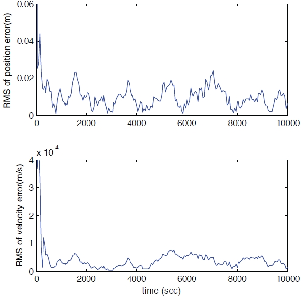
Fig. 12 shows the errors in position of chief satellite when the GPS observations are renewed once in 1 hour. In the figure, we can see that the errors are accumulated from several ten meters to several hundred meters, and reduced up to 1 meter level due to determination of position through the GPS. The results of filtering reflecting these effects are the same as shown in Fig. 13, and we can confirm that the filtering was well performed similar to the previous example. The magnitude of errors in three-dimensional space is represented as RMS in Fig. 14, and in this figure the upper part shows the errors in determination of relative position, and the lower part shows the errors in determination of relative velocity. In order to compare the impact of cycle for determination of position of chief satellite under the same condition, in Table 3, we represented the case that the determination of position of chief satellite based on GPS data is performed every 30 seconds at 10 km distance, together with the case that it is performed every 1 hour. In case of 30 seconds, the results of Table 2 were entered once again, and all values are ones stabilized from after 500 seconds. In case that the information on determination of position of chief satellite is received every 1 hour, the precision level of determination in position and velocity is 9.3 mm and 32 μm, respectively.
Compared to the case that the determination of position of chief satellite was performed every 30 seconds, the precision level became lower by 16% for position, and by 100% for velocity, but there were no differences in the order, and it was possible to determine the relative position with a similar precision level.
We implemented the algorithm to determine the relative position using an inter-satellite laser. In this study, we used only the observation values corresponding to relative position, and did not use the observation information corresponding to velocity. However, the velocity values obtained on the basis of dynamic model were used to remove a drift caused by the characteristic of laser using the LPF. Although the laser system has a small measurement noise, but when it is applied to a moving satellite, a drift larger than measurement noise occurs. So, it is impossible to determine the precise relative position only based on observation values. Therefore, it is meaningful to implement the system to determine the precise relative position by applying the observation values and dynamic model to the EKF algorithm properly. The precision level in determination of relative position obtained in this study implies that the relative velocity with an appropriate precision level can be obtained even not observing the relative velocity.
Comparing the precision level with the same 1 km, in existing study that used GPS, it was represented as millimeter level, and in another study that used the laser radar, it was represented as centimeter level. On the contrary, in this study it was improved up to sub-millimeter level. Because the closer the distance becomes, the less the impact of angular errors are, it is possible to perform a precise determination, and also in this study, it was confirmed that a real-time determination of precise relative position was possibly performed at several millimeter level even at the distance 10 km farther compared to the study that used the existing laser. In addition, as a result of simulation for the case that the GPS data was not received for long hours, notwithstanding that the determination of relative position of chief satellite was performed every 1 hour, the precision level in determination of relative position did not drop greatly. These results mean that if the determination of orbit of chief satellite is realized at 1m level, the errors caused by orbit propagation for long hours do not affect greatly the determination of relative position using the laser. These results show the diverse applicability of algorithm to determine the relative position using the synthetic wavelength of femtosecond laser.