A number of existing and emerging concepts for formulating solution algorithms applicable to multidisciplinary inverse problems involving aerodynamics, heat conduction, elasticity, and material properties of arbitrary three-dimensional objects are briefly surveyed. Certain unique features of these algorithms and their advantages are sketched for use with boundary element and finite element methods.
A mathematically well-posed analysis problem is considered solvable when provided governing equation(s), shape(s) and size(s) of the domain(s), boundary and initial conditions, material properties of the media contained in the domain, and internal sources and external forces or inputs. When any this information is missing, the field problem becomes incompletely defined (ill-posed) and is of an indirect (or inverse) type [1]. The inverse problems can therefore be classified as determination of unknown governing equations, shapes and sizes, boundary/initial values, material properties, and sources and forces. The inverse problems can be solved if sufficient amount and type of additional information is provided. Following is a very brief survey of some of the solution methods for multidisciplinary inverse problems that have been researched in the Multidisciplinary Analysis, Inverse Design, Robust Optimization and Control (MAIDROC) Laboratory at FIU.
2 Aerodynamic Shape Inverse Design
Aerodynamic shape inverse design involves the ability to determine the shape of an aerodynamic configuration that will satisfy the governing flow-field equation(s) while enforcing specified (desired or target) surface pressure distribution and certain geometric constraints.
Aerodynamic shape optimization design involves the ability to determine the shape of an aerodynamic configuration that will satisfy the governing flow-field equation(s) while extremizing global aerodynamic parameters (coefficients of lift, drag, moment) and satisfying certain geometric and/or flow-field constraints [2-12].
Aerodynamic shape inverse design methods typically require significantly fewer analyses of flow-fields during the iterative design process than are typically required when using an aerodynamic shape optimization approach. However, aerodynamic shape inverse design methods require designers with adequate experience to specify a good surface target pressure distribution.
2.1 Choosing Target Surface Pressure Distribution
Aerodynamic shape inverse design enforces desired pressure distribution on the unknown object’s surface often without any direct evaluation criterion available to judge the effects of this pressure distribution on the corresponding global design objectives such as lift, drag, and moment. Since the inverse shape design enforces the specified (target) surface pressure distribution, the common dilemma is the choice of the "best" target pressure distribution.
Specifically, it would be desirable to specify such pressure distribution on the surface of the yet unknown threedimensional object so that it maximizes the aerodynamic efficiency by minimizing the aerodynamic drag. Therefore, any candidate target surface pressure distribution should first be checked for possibly causing flow separation before it is actually enforced in the aerodynamic shape inverse design process. A number of approaches have been published to detect flow separation utilizing information from the computed viscous boundary layer parameters [13]. These flow separation detection methods are based mainly on two-dimensional, laminar, incompressible boundary layer analysis. Thus, they require knowledge of the pattern of streamlines on a three-dimensional body surface which is impossible to determine in an a priori fashion since the shape of the body is yet unknown. A typical approach has been to calculate an inviscid flow around an initially guessed shape of the three-dimensional body, determine surface streamlines, apply a two-dimensional boundary layer calculation in a strip fashion along each three-dimensional streamline, and then use one of these known boundary layer separation detection criteria. However, it would be very desirable to avoid a need for boundary layer calculations altogether and use only the information from an inviscid flow analysis in order to detect locations of flow separation.
2.2 Sih’s Concept for Detecting Flow Separation
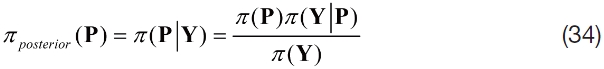
One very fast method for detecting flow separation in case of incompressible and compressible, two-dimensional and three-dimensional, steady and unsteady flows is based on the postulate that “separation occurs at the location near the boundary where the rate of increase of potential energy density is a local maximum” [14]. Actually, it is more practical to search for locations where the rate of change of flow kinetic energy reaches its minimum [14] since the surface flow kinetic energy variation can be calculated from the surface pressure distribution by assuming that pressure does not change across a viscous boundary layer.
The following general analytic formulation (Eq. 1) is valid for flow separation detection based on a minimum variation of the kinetic energy rate [15] in case of multi-dimensional, isothermal, adiabatic, steady and unsteady, compressible and incompressible. Here, Ek is the kinetic energy per unit volume,
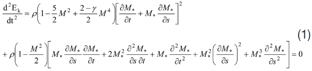
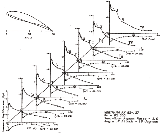
This exceptionally fast and versatile flow separation detection concept was tested against experimental results for a low Reynolds number incompressible flow over a rectangular wing at different angles of attack [16]. The experimental results are summarized in Fig. 1 where S and R designate separation and reattachment points, respectively [16]. The corresponding plots of quasi two-dimensional variation of the kinetic energy rate are shown in Fig. 2 [15] demonstrating the validity of Sih's concept [14] for detection of separation points since locations of minima of the kinetic energy rate along each airfoil section corresponds to the locations of separation observed during the wind tunnel experiment.
It should be pointed out that Fig. 2 indicates existence of narrow laminar separation along the leading edge. This was not mentioned in the original report by the experimentalists [16], but was afterwards privately acknowledged as actually observed.
Additional comparisons between the experimentally measured flow separation locations and the flow
separation locations were presented by Dulikravich [15] for incompressible flows around circular and elliptic cylinders at different Reynolds numbers, and around a transonic airfoil with a shock induced separation and a narrow leading edge separation due to manufacturing imperfection when building the airfoil that was experimentally tested.
2.3 Elastic Membrane Motion Concept for Inverse Determination of Unknown Shapes
There are many algorithms for inverse determination of unknown shapes, but they are almost always highly specialized for a particular mathematical model. Besides, many of the existing methods require that initially guessed shape be quite close to the finally determined shape. Furthermore, they are often not applicable to threedimensional configurations and cannot make use of the commercially available analysis software because such licensed software cannot be altered, while the ultimate need of a shape designer is to utilize the existing field analysis commercial software in the inverse shape design with no need for modifications of such software. Consequently, an acceptable approach to inverse shape design is to use a simple, fast and robust master code that calculates corrections to the iteratively evolving shape of an object, while utilizing a commercially available field analysis code to evaluate each intermediate shape.
One such concept of inverse shape design will be briefly demonstrated in case of an inverse shape design of an airplane wing at arbitrary speed. The basic idea due to Garabedian and McFadden [17] is that surface of the aerodynamic flight vehicle that should have a specified surface pressure distribution can be heuristically modeled as damped elastic membranes subject to time-dependent forcing functions. If each point of the wing surface membrane is loaded with a point-force, ΔCp, proportional to the local difference between the calculated and the specified coefficient of surface pressure, the wing surface membrane will iteratively deform until it assumes a steady position that experiences zero forcing function at each of the membrane points. The governing equations for an elastic membrane could be of the standard spring-damper-mass forced vibration type and have traditionally been discretized using finite differences and integrated numerically [18-20]. However, when using non-linear flow-field analysis such as Navier-Stokes solvers, this iterative inverse shape design method converges slowly. A semi-analytical method for integration of such differential equations has been developed that is based on Fourier series and converges much faster [21-23].
2.3.1 Three-Dimensional Elastic Membrane Concept with Fourier Series Integration
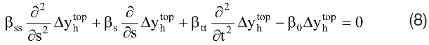
This formulation will be explained for the case of inverse shape design of an isolated three-dimensional airplane wing at arbitrary flight speed. Wing surface can be described by two surface coordinates, s and t. The s-coordinate starts at the lower trailing edge point and follows an airfoil shape in a clockwise direction ending at the upper trailing edge point. The second surface-following coordinate, t, begins at the wing root and goes span wise to the wing tip and then returns along the upper surface of the wing back to the wing root. The surface following coordinates should be scaled so that the line s = π occurs at the leading edge of the wing, the line s = 2π occurs at the trailing edge of the wing, and the line t = π occurs at the wing tip. Notice that coordinate directions s and t are not necessarily orthogonal to each other. Evolution model of the top surface of the wing can then be assumed to be of the form [21-23]
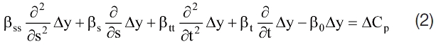
with a similar evolution model of the bottom surface of the wing. Here, coefficients β are the user specified constants controlling the rate of damping and convergence to the steady state solution. The arbitrarily varying globally periodic aerodynamic forcing function,
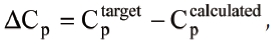
can be represented using the Fourier series expansion of the form
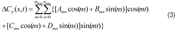
The particular solutions of the linear partial differential equations (19) and (20) can be assumed to be of the similar Fourier series form.
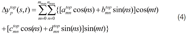
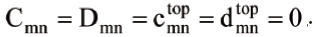
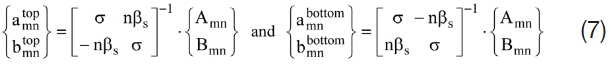
with a similar expression for the bottom surface of the wing. Substitution of Eq. 3 and Eq. 4 into Eq. 2 for the top surface of the wing yields
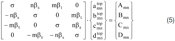
with the similar expression for the lower surface of the wing. Here,

For the special case where the pressure distribution and wing deformation are symmetrical about the wing root symmetry plane, t = 0, it follows that
Thus, t-direction damping should not be used (βt = 0) for span wise symmetric configurations. Consequently,
The differing Fourier coefficients in the particular solutions on the upper and lower surfaces give rise to a gap formation along the leading and trailing edges of the wing. There will also be a slope discontinuity that develops at the leading and trailing edges. Series of homogeneous solutions to the shape evolution Eq. 2 and its counterpart on the lower surface of the wing are used to overcome these gaps. Specifically, on the top surface of the wing, the homogeneous solution should satisfy
Then, on the upper surface of the wing, the y-coordinate correction due to the homogeneous solution is
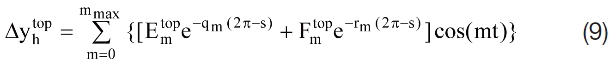
where qm and rm are analytic functions of the b coefficients and the mode number, m. Similarly, on the bottom surface of the wing,
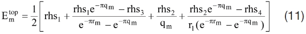
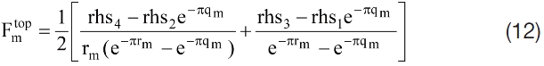
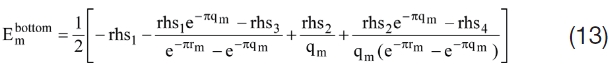
Combining the boundary conditions (equal values of homogeneous solutions and slopes given by the homogeneous solutions at the leading edge and the trailing edge points) results in analytic equations for E and F coefficients in each mode, m.
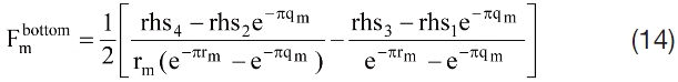
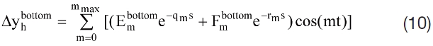
Finally, after combining homogeneous and particular solutions, analytic expressions for geometry corrections are
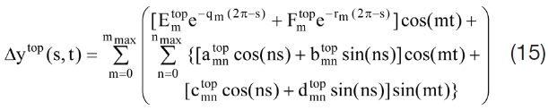
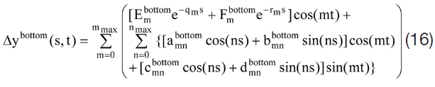
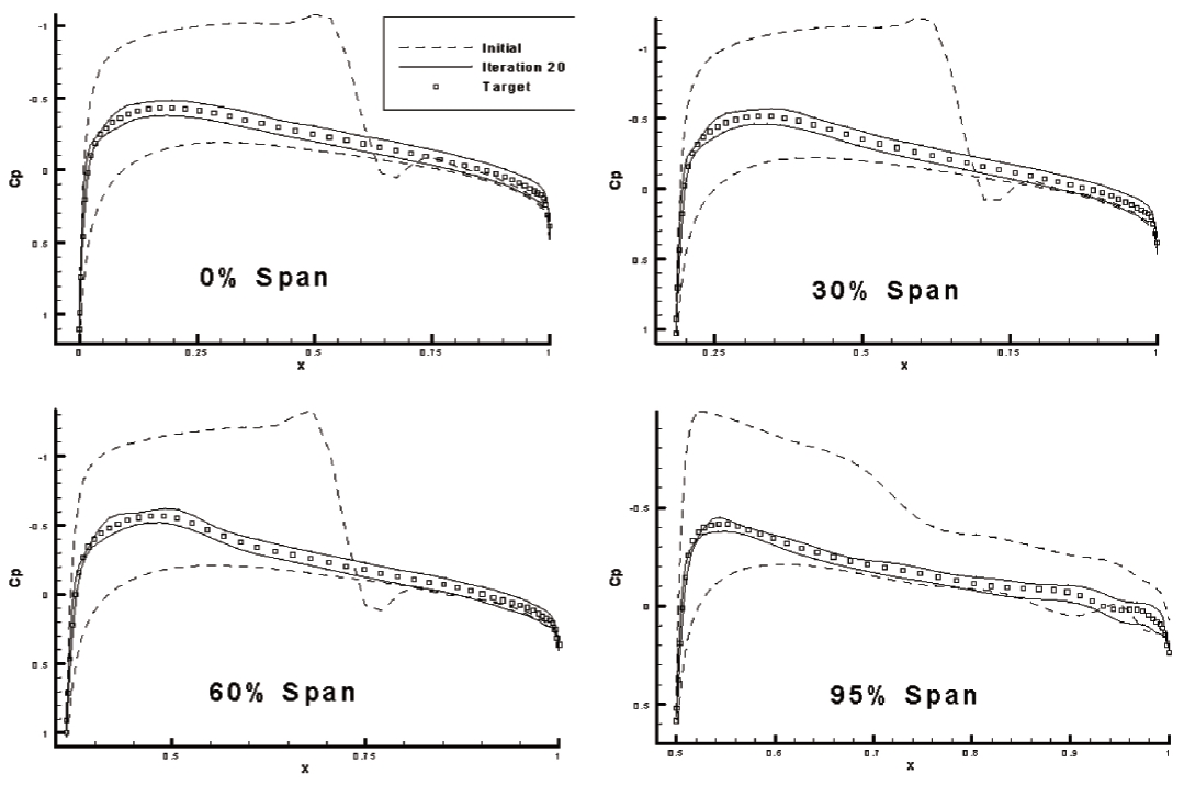
An example of application [22] of the Fourier series formulation of the solution of the elastic surface membrane concept is given in Fig. 3. The objective was to test the Fourier technique’s ability to simultaneously modify a transonic wing’s span wise distribution of thickness, camber, twist, and dihedral seeking to design a fully subsonic wing from a wing with an initial shock wave at the flight Mach number M = 0.8. The wing planform had a taper ratio of 0.5, leading edge sweep angle of 14.03 degrees, zero trailing edge sweep, and semi-span of two times the root chord length. The initial guess had a NACA 0012 airfoil shape at +5.0 degrees angle of attack. The target pressure distribution corresponded to a non-lifting wing with a NACA 0009 airfoil.
This shape inverse design method converges monotonically to a smooth shape even for a very irregular specified distribution of surface pressures and for a significantly wrong initial guess for the geometry. Thus, it is much more cost effective to use the optimization algorithms for actual constrained optimization of the global aerodynamic parameters such as coefficients of lift, drag and moment, instead of using optimization to achieve inverse shape design by enforcing user specified surface pressure distributions. Notice that this inverse shape design method can readily be applied not only in aerodynamics/fluid dynamics, but also in three-dimensional heat conduction [24], elasticity, magnetostatics and electrostatics fields.
2.4. Determining Number, Sizes, Shapes and Locations of Inclusions
During the past two decades, our research team has been developing a unique inverse shape determination methodology that utilizes an optimization algorithm as a tool to determine the proper number, sizes, locations and shapes of inclusions in heat conduction and elasticity problems [25-30]. For example, the designer needs to specify both the desired temperatures and heat fluxes on the hot surface, and either temperatures or convective heat coefficients on the guessed internal coolant passage walls. The designer must also provide an initial guess to the total number, sizes, shapes, and locations of the internal coolant flow passages. Afterwards, the design process uses a constrained optimization algorithm [31,32] to minimize the difference between the specified and computed hot surface heat fluxes by automatically relocating, resizing, reshaping and reorienting the initially-guessed coolant passages. All unnecessary coolant flow passages will be automatically reduced to very small sizes and eliminated while honouring the specified minimum distances between the neighbouring passages and between any passage and the thermal barrier coating if such exists. This type of computer code is highly economical, reliable, and geometrically flexible, especially when it utilizes the boundary element method (BEM) that does not require generation of the interior grid and is non-iterative. The methodology has been successfully demonstrated on coated and non-coated turbine blade airfoils, scramjet combustor struts, three-dimensional coolant passages in the walls of rocket engine combustion chambers and axial gas turbine blades [25-30].
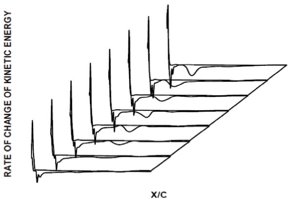
This type of inverse problems requires that numerical error be reduced until it becomes at least one or two orders of magnitude lower than in case of solving a related forward (analysis) problem. Otherwise, an illusion of non-unique solutions can be created, while these solutions are merely a consequence of the under-iterated process of minimizing the least square difference between the target over-specified boundary conditions and the calculated conditions (Eq. 17).
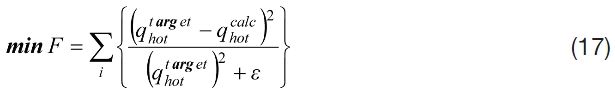
where
When guessing that there should be three smaller holes (left figure) and enforcing the overspecified boundary
conditions (constant temperature and constant heat flux on the outer ? hot boundary, two holes shrunk to points indicated by arrows, while third hole grew and positioned itself in the correct central location. Results in the left figure correspond to a solution that converged to 0.1 percent of integrated flux error. Results on the right show the same three-hole initial configuration and their locations and sizes corresponding to the integrated heat flux error of 1.86 percent [27].
3. Determination of Steady Boundary Conditions on Inaccessible Boundaries
3.1 Determining Steady Boundary Conditions Using Boundary Element Method
In elastostatics, a problem is well-posed when the geometry of the three-dimensional object is known and either displacement vectors, {u}, or surface traction vectors, {p}, are specified everywhere on the surface of the object. The elastostatic problem becomes ill posed when either a part of the object's geometry is not known or when both {u} and {p} are unknown on certain parts of the surface. Both types of inverse problems can be solved if both {u} and {p} are simultaneously provided on certain surfaces of the body [33].
Similarly, determination of unknown steady thermal boundary conditions when temperature, heat flux, or heat transfer coefficient data are unavailable on certain boundaries is a common class of inverse problem [34-37]. The missing boundary conditions can be found if both temperature and heat flux are available on other, accessible boundaries or at a finite number of points within the domain. A very simple non-iterative approach to solving such inverse problems is possible when using Boundary Element Method (BEM) to solve the governing equations. We will sketch the BEM in case of heat conduction equation for the steady-state temperature distribution; T(x), in a solid isotropic domain Ω bounded by the boundary Γ is given by

Here,
Here,

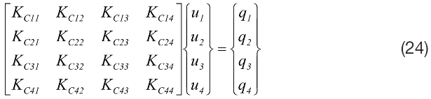
where [H], [G] and [R] are the geometric coefficient matrices. For example, if at two vertices (1 and 3) of a quadrilateral surface panel both
are known, while at the remaining two vertices (2 and 4) neither quantity is known, the BIE equation set begins as [33]
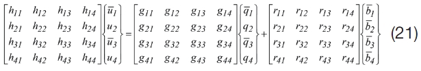
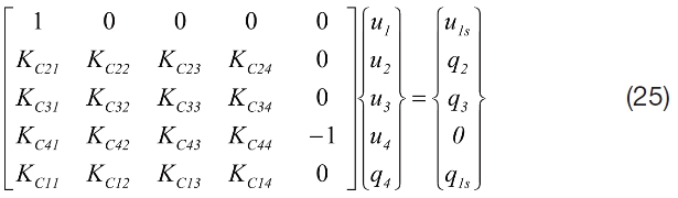
For a well-posed boundary condition problem, every point on the boundary is given either one Dirichlet, one Neumann or one Robin boundary condition assuming that internal heat source distribution is known. Additional equations may be added to this equation set if temperature measurements are known at certain locations within the domain. The known nodal variables are then multiplied by their respective coefficient matrix terms and transferred to the right hand side [33-37]. Similarly, all unknown nodal variables are multiplied by their respective coefficient matrix terms and transferred to the left hand side.
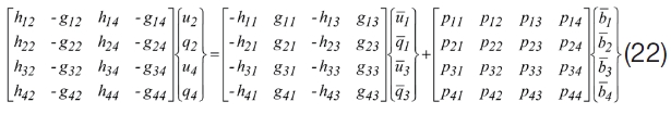
Notice that the entire right hand side is known and can be condensed into a vector {F}. The result is a standard linear matrix problem of the general type [A]{X}={F}. In general, the geometric coefficient matrix [A] will be non-square and highly ill-conditioned. Singular Value Decomposition (SVD) methods [38], are widely used for solving linear least squares problems of this type. Thus, by using an SVD type algorithm and truncating singular values that are corrupted by round-off error, it is possible to solve for the unknown surface temperatures and heat fluxes simultaneously, very accurately, and non-iteratively.
3.1.1 Inverse Determination of Spatially Varying Heat Convection Coefficient
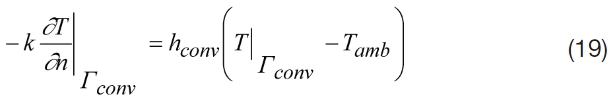
As a very useful by-product of this inverse method, the inversely determined surface temperatures and heat fluxes yield values of previously unknown convective heat transfer coefficients (see Eq. 19). Thus, rather than trying to evaluate the surface variation of the convective heat transfer coefficient by using flow-field analyses, it is possible to treat the heat convection coefficient determination problem as an ill-posed heat conduction problem solved only in the solid that is in contact with the moving fluid. Here, no thermal data needs to be available on parts of the boundary exposed to a moving fluid, while temperatures and heat fluxes are available on other boundaries or inside the solid. Results were excellent for Biot numbers from 0.01 to 100 [39].
3.2 Determination of Steady Boundary Conditions Using Finite Elements
The same general concept used with BEM formulation is also applicable when using the FEM formulation in simultaneous prediction of steady thermal and elasticity boundary conditions. FEM formulation with Galerkin’s method [40-43] after assembling all element equations results in two linear algebraic systems that could be expressed (in case of no heat sources) as

Here, [
In the case of an ill-posed problem, thermal and elasticity boundary conditions will not be known on some parts of the boundary. For example, in three-dimensional heat conduction while using a tetrahedral (three-dimensional) finite element, one could specify both the temperature, us, and the heat flux,
A similar procedure is also applied to the elasticity system of equations [40-43] where thermal stresses are accounted for in the vector {
3.3 Regularization Formulations
In any iterative solution algorithm, such as FEM, if the iterative matrix is highly ill-conditioned, a regularization method needs to be applied to the solution of the systems of equations in an attempt to increase the method’s tolerance to possible measurement errors in the over-specified boundary conditions. Here, we consider the regularization of the inverse heat conduction problem. The general form of a regularized system is given as [40]
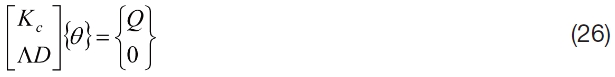
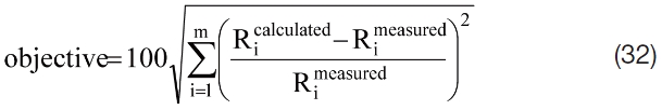
Solving Eq. 26 in a least squares sense minimizes the following error function.

This represents the least squares minimization of the residual plus a penalty term. The form of the damping matrix determines what penalty is used and the damping parameter, ?, weights the penalty for each equation. These weights should be determined according to the error associated with the respective equation. Notice that [
In order to minimize the error in the domain of the object, this regularization method uses Laplacian smoothing of the unknown temperatures and displacements only on the boundaries where the boundary conditions are unknown. A penalty term can be constructed such that curvature of the solution on the unknown boundaries where boundary conditions are unknown is minimized along with the residual.

For problems that involve unknown vector fields, such as displacements, Eqn. 28 is modified to smooth a certain component of the field.

Here, the normal component of the vector displacement field {

three-dimensional problems, [
For each boundary element on unknown boundary we transform Laplace’s equation to natural surface-following coordinates, discretize Laplace’s equation using Galerkin’s method, compute local damping matrix [
can be used to solve these normalized systems, but such systems are usually highly ill-conditioned. Iterative methods are difficult to use in practice since they require good preconditioners for fast convergence. Use of static condensation method for decreasing the sparseness of the matrix and then use of a dense rectangular solver such as SVD to solve for the unknowns on the boundary is also an option [42].
3.4 Inverse Determination of Unsteady Surface Temperature on a Three-dimensional Object
An unsteady version of the same spectral finite element code for determination of steady temperatures and heat
fluxes on inaccessible surfaces has also been successfully demonstrated [43].
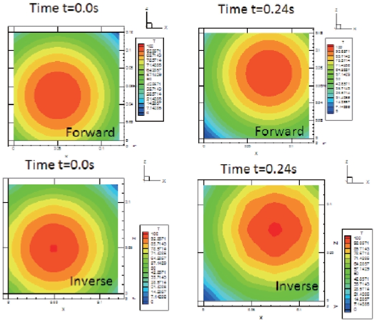
In an example where a strong laser beam is impinging on a top surface of a square plate and travels steadily along the diagonal (Fig. 6), temperature on the top surface is so high that it could melt surface temperature sensors. Therefore, temperature is safely measured on the bottom surface of the plate. From the known heat flux distribution on the top surface and the measured unsteady temperature field on the bottom surface, an unsteady three-dimensional temperature filed can be calculated (assuming that side walls are adiabatic). As a byproduct, we also get the unsteady temperature distribution on the top surface. This well-posed analysis problem can then be converted into an inverse problem where nothing is known on the bottom surface, while top surface has specified unsteady temperature and heat flux distributions.
4. Inverse Determination of Physical Properties of the Media
An increasingly important application of inverse methodologies is the determination of physical properties (thermal conductivity, electric conductivity, specific heat, thermal diffusivity, viscosity, magnetic permittivity, etc.) of the media. These properties could depend on certain field variables (temperature, pressure, density, frequency, etc.). Many applications do not allow the destruction of an object in order to extract and test a specifically shaped and sized test sample. Thus, inverse determination of the physical properties is very popular in the non-destructive evaluation community.
4.1 Inverse Problem Formulation for Determining Modulus of Elasticity Variation
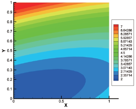
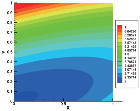
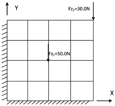
In this section, we consider the inverse determination of a spatially varying modulus of elasticity in a load bearing structure. For simplicity, we will work with a 1.0 m x 1.0 m plate that is fixed on two ends and under two transverse point loads as shown in Fig. 7. The plate thickness is 0.2 m. The forward (analysis) problem can be solved with a straightforward application of the finite element method. In our case, this involved discretizing the plate with 16 four-node isoparametric elements of the shear deformable displacement formulation (Mindlin plate elements) [44] as shown in Fig. 7. The modulus of elasticity,

The forward (analysis) problem was created by setting {
The initial guess for the values of the modulus of elasticity was {
4.2 Inverse Determination of Temperature-dependent Thermal Conductivity
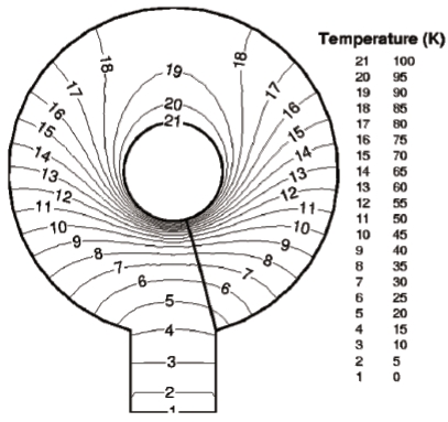
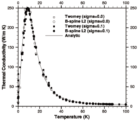
If measured values of heat fluxes (or convection heat transfer coefficients) are available everywhere on the surface of an arbitrarily shaped solid, then Kirchhoff’s transformation can be used to convert the governing steady heat conduction equation with temperature-dependent thermal conductivity into a linear boundary value problem that can be solved via BEM for the unknown Kirchhoff’s heat functions on the boundary [45]. Given several boundary temperature measurements, these heat functions are then inverted to obtain the temperature variation of thermal conductivity at the points where the over-specified (temperature and heat flux) measurements were taken. Several different inversion procedures were attempted, including regularization, finite differencing, and least squares fitting with a variety of basis functions. The program is very accurate when the data is
without error, and it does not excessively amplify input temperature measurement errors when those errors are less than 5% standard deviation. The algorithm was found to be less sensitive to measurement errors in heat fluxes than to errors in temperatures. The accuracy of the algorithm was greatly increased with the use of a priori knowledge about the thermal conductivity basis functions.
The experimental part of this inverse method requires one temperature probe and one heat flux probe that need to be moved from point-to-point on the surface of an arbitrarily shaped and sized specimen (Fig. 10). Thus, this method is directly applicable to field testing, since special test specimens do not need to be manufactured. This inherently multi-dimensional method could still use temperature measurements at interior points if additional accuracy is desired (Fig. 11).
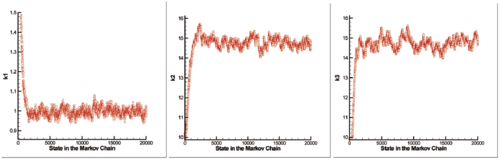
4.3 Bayesian Approach to Inverse Determination of Temperature-Dependent Thermal Conductivity
The solution of the inverse problems within the Bayesian framework can be recast in the form of statistical inference from the
where Y is the measurements and T(P) is the solution of the direct (forward) problem. The model for the unknowns that reflects all the uncertainty of the parameters without the information conveyed by the measurements is called the prior model. The formal mechanism to combine the new information (measurements) with the previously available information (prior) is known as the Bayes’ theorem. Therefore, the term Bayesian is often used to describe the statistical inversion approach, which is stated as [46]
where π
4.4 Inverse Design of Metallic Alloys for Specified Performance
Inversely designing new alloys for specific applications involves determining concentrations of alloying elements that will provide, for example, specified tensile strength at a specified temperature for a specified length of time [47-49]. This represents an inverse problem which can be formulated as a multi-objective optimization problem with a given set of equality constraints. This approach allows a materials design engineer to design a precise chemical composition of an alloy that is needed for building a particular object. This inverse method uses a multi-objective constrained evolutionary optimization algorithm [50,51] to determine not one, but a number of alloys (Pareto front points) each of which will satisfy the specified properties while having
different concentrations of each of the alloying elements. This provides the user of the alloy with an additional flexibility when creating such an alloy, because he/she can use the chemical composition which is made of the most readily available and the most inexpensive chemical elements. It should be pointed out that the inverse problem of determining alloy chemical composition is different from a direct optimization problem of designing alloys that will have extreme properties. This alloy design methodology does not require knowledge of metallurgy or crystallography and is directly applicable to alloys having arbitrary number of alloying elements.
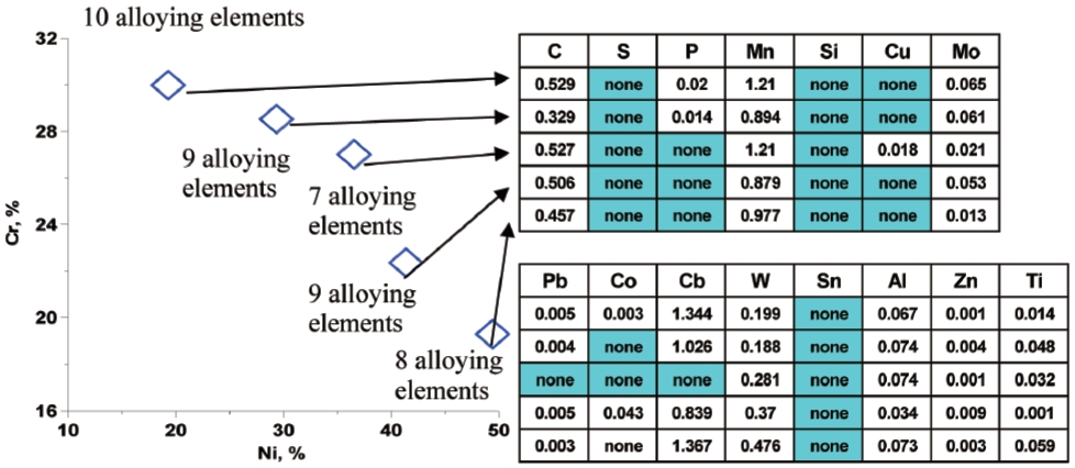
A design example is presented for Ni-based steel alloys, although the method is applicable to inversely designing chemical concentrations of arbitrary alloys. In this example, a maximum of 17 candidate alloying elements were considered (Cr, Ni, C, S, P, Mn, Si, Cu, Mo, Pb, Co, Cb, W, Sn, Al, Zn, Ti). The following three desired properties of the alloys were specified: tensile strength σ
Results of this multi-objective constrained optimization task are given in Fig. 13 by presenting five Pareto optimized alloys on the left hand side in terms of their concentrations of Ni and Cr, and the concentrations of the remaining 15 candidate alloying elements for each of the five Pareto optimized alloys given on the right hand side. Each of the five inversely designed alloys satisfies the three specified alloy properties, while providing Pareto-optimized minimum use of seven alloying elements. It is fascinating to realize
that optimized concentrations of some of the remaining 15 candidate alloying elements were found to be negligible although they are currently widely used in such alloys, thus eliminating these elements as potential candidates for forming these types of steel alloys. Consequently, the number of alloying elements that actually needs to be used to create an alloy with the three specified properties could be as low as 7 instead of 15 (in addition to Ni and Cr). This is highly attractive for practical applications where regular supply, storage, and application of a large number of different pure elements are considered impractical, costly and financially risky.
5. Summary and Recommendations
A number of concepts and applications have been briefly exposed for formulating and solving a variety of seemingly unsolvable (ill-posed) problems. A common result of most of these analytical formulations and their discretized versions are highly ill-conditioned matrices representing systems of linear algebraic equations. Boundary element methods typically result in dense ill-conditioned matrices and finite element methods typically result in sparse illconditioned matrices. Existing algorithms for solution of both types of ill-conditioned matrix problems are not sufficiently fast and accurate when applied to arbitrary three-dimensional domains, unsteady problems, and especially multidisciplinary problems. Another persistent issue in the numerical solution of inverse problems is the control of numerical errors in the iterative solution methods. Further innovative research is needed in the development of appropriate regularization concepts that do not deteriorate the accuracy of the solution and that are applicable to large initial and boundary data errors.

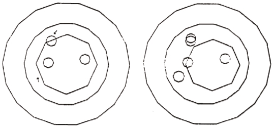
![Experimental results [16] for coefficient of pressure distributions on upper and lower surface of a rectangular wing at 18 degrees angle of attack in a free stream Mach number M = 0.1 and Reynolds number Re = 80,000. Letters S, T and R designate observed locations of flow separation, transition and reattachment.](http://oak.go.kr/repository/journal/11779/HGJHC0_2012_v13n4_405_f001.jpg)
![A shocked transonic wing was redesigned [22] into a shock-free wing using Fourier series formulation of the elastic membrane concept and a flow-field analysis code solving Euler equations.](http://oak.go.kr/repository/journal/11779/HGJHC0_2012_v13n4_405_f003.jpg)
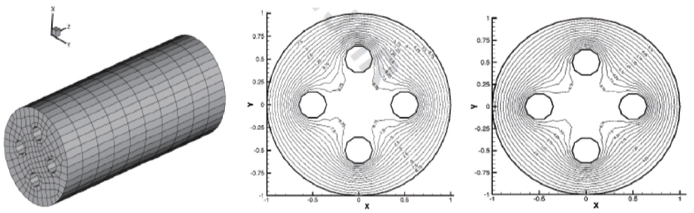
![An example of inverse determination of temperatures on surfaces of interior holes and in the entire three-dimensional cylinder when outer surface temperatures and heat fluxes are known, but nothing is known onside the cylinder nor on the surfaces of the four holes: finite element grid (left), calculated isotherms when temperature is known on outer and inner surfaces (middle), calculated isotherms when only outer surface temperatures and heat fluxes are known (right) [42].](http://oak.go.kr/repository/journal/11779/HGJHC0_2012_v13n4_405_f005.jpg)
![Actual temperature evolution on the bottom surface of the plate (top figures) and inversely determined temperature distribution on the bottom of the plate (bottom figures) in case when unsteady temperature and heat flux were specified on the top surface and nothing was known on the bottom surface of the plate. Test case assumed no measurement errors [43].](http://oak.go.kr/repository/journal/11779/HGJHC0_2012_v13n4_405_f006.jpg)
![Distribution of E(x, y) used for the forward solution [44]](http://oak.go.kr/repository/journal/11779/HGJHC0_2012_v13n4_405_f008.jpg)
![Predicted E(x, y) using measured Fz and M on the boundaries [44]](http://oak.go.kr/repository/journal/11779/HGJHC0_2012_v13n4_405_f009.jpg)
![Isotherms predicted by a non-linear BEM based on surface measurements of temperature and heat flux for a keyhole shaped object that was internally heated and made of copper [45].](http://oak.go.kr/repository/journal/11779/HGJHC0_2012_v13n4_405_f010.jpg)
![Inversely calculated variation of thermal conductivity for the specimen from Fig. 10. Results with zero measurement errors and with 10 percent standard deviation measurement error [45].](http://oak.go.kr/repository/journal/11779/HGJHC0_2012_v13n4_405_f011.jpg)
![States of the Markov chain with standard deviation σ = 0.05 for inversely determined components k1 (left), k2 (middle) and k3 (right) of the orthotropic heat conduction coefficient [46].](http://oak.go.kr/repository/journal/11779/HGJHC0_2012_v13n4_405_f012.jpg)
![An example of determining alloying elements and their concentrations for inversely designed Ni-base alloys with three specified proper ties, while minimizing the cost of raw material [49].](http://oak.go.kr/repository/journal/11779/HGJHC0_2012_v13n4_405_f013.jpg)