The state-of-the-art techniques in multicore timing analysis are limited to analyze multicores with shared instruction caches only. This paper proposes a uniform framework to analyze the worst-case performance for both shared instruction caches and data caches in a multicore platform. Our approach is based on a new concept called address flow graph, which can be used to model both instruction and data accesses for timing analysis. Our experiments, as a proof-of-concept study, indicate that the proposed approach can accurately compute the worst-case performance for real-time threads running on a dual-core processor with a shared L2 cache (either to store instructions or data).
Multicore chips can offer many important advantages such as higher throughput, energy efficiency and density. However, to safely exploit multicore chips for real-time systems, especially hard real-time systems, it is crucial to accurately obtain the worst-case execution time (WCET). This, however, is a very challenging task, due to the enormous complexity caused by inter-thread interferences in accessing shared resources in multicores, such as shared caches.
In the last two decades, WCET analysis has been actively studied, and a good review regarding the stateof- the-art can be found at [1]. Most of the prior research efforts, however, focus on WCET analysis for uniprocessors [2-6], which cannot be used to estimate the WCET for multicore processors due to their inability to estimate the worst-case inter-thread interferences in shared resources such as caches.
There are also some studies on WCET analysis for multi-tasking uniprocessors [7-10], which, however, still cannot be applied to estimate inter-thread cache conflicts on multicore chips. This is because in a multi-tasking uniprocessor system, threads (i.e., tasks) are typically assigned by different priorities and are preemptive. When preemption occurs, the cache memories are taken over by a higher prioritized thread solely and later given back to the lower prioritized thread when the higher prioritized thread finishes. Therefore, the preemption of a thread implicitly causes the preemption of the cache memories simultaneously, making it possible to find such preemption points, at which the higher prioritized threads will produce the worst cache related preemptive delay (CRPD). In a multicore model, however, threads are running in parallel and cannot preempt each other across different cores. Thus, the interferences among threads are solely determined by the timing order information of all the cache accesses from all the threads. So, the worst-case cache related delay for a given thread is determined by a set of interference points caused by the accessing sequences of all the cache accesses and from all the threads. This essential difference makes existing analysis techniques for multitasking uniprocessors [7-10] not applicable to the multicore WCET analysis.
Recently, there have been an increasing number of research efforts on real-time scheduling for multicore platforms [11,12]. However, all these studies basically assume that the worst-case performance of real-time threads is known a priori. Therefore, it is critical to develop new timing analysis techniques to reasonably estimate the WCET of real-time threads running on multicore processors.
To the best of our knowledge, the state-of-the-art timing analysis techniques for multicore processors studied in recent work [13-15] are unable to estimate the worst-case performance of shared instruction caches of multicores. While these studies [13-15] have made initial contributions towards the timing analysis of multicores, their inability to analyze shared data caches fundamentally limits the applicability of these methods, considering the widespread use of data caches in multicore processors and their significant impact on the execution time, including the WCET. To address this problem, this paper proposes to use an address flow graph (AFG) to conduct a timing analysis, which can be generally applied to not only instruction caches, but also data caches as well as unified caches. Also, to the best of our knowledge, this paper is the first work to extend the implicit path enumeration technique (IPET) [4,5] from uniprocessors to multicores, and the beauty of our approach is that both the path analysis (of single core) and shared cache analysis are based on IPET, which can implicitly compute the WCET of real-time tasks running on a multicore chip safely and accurately by considering all possible paths of each and all concurrent threads, as well as all possible interactions among them.
II. ASSUMED MULTICORE ARCHITECTURE
In a multicore processor, each core typically has private L1 instruction and data caches. The L2 (and/or L3) caches can be shared or private. While private L2 caches are more time-predictable in the sense that there are no inter-thread L2 cache conflicts, they suffer from other deficiencies. First, each core with a private L2 cache can only exploit separated and limited cache space. Second, separated L2 caches will increase the cache synchronization and coherency cost. Moreover, a shared L2 cache
architecture makes it easier for multiple cooperative threads to share instructions and data, which become more expensive in separated L2 caches. Therefore, in this paper, we will study the WCET analysis of multicore processors with shared L2 caches (by contrast, the WCET analysis for multicore chips with private L2 caches is a less challenging problem).
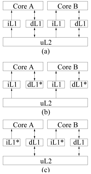
In this paper, we focus on examining the WCET analysis for a dual-core processor with a shared L2 cache, although our approach can also be generally applied to multicore processors with a greater number of cores. Fig. 1 shows a processor, where each core has private L1 instruction and data caches, and shares a unified L2 cache. In this work, we focus on analyzing the inter-thread interferences caused by both instruction and data streams. Specifically, we assume the L1 data (instruction) cache in each core is perfect when analyzing the instruction (data) cache, as depicted in Fig. 1b and c, respectively. Due to the common analysis framework of both instruction and data interferences, our approach can also be easily applied to a unified shared cache with both data and instruction accesses, which will be examined in our future work.
III. COMPUTING THE WORST-CASE DELAY OF INTER-THREAD CACHE INTERFERENCES
Cache related delay (CRD) is the delay due to the presence of cache memories, which makes the latency of accessing an instruction or data fluctuate, depending on whether or not the instruction or data can be found from a particular level of cache. Generally speaking, the CRD problem can be tackled in at least two different ways. One approach is to statically classify each instruction, thus the upper bound latency can be derived for each instruction, which is then integrated with pipeline analysis and path analysis to derive the WCET [2]. Another approach is to use the IPET [4,5], which is built upon constraint programming to bind the CRD and then leverage integer linear programming (ILP) to compute the CRD and the WCET. This paper adopts IPET to compute WCET. However, the original IPET [4,5] was proposed for timing analysis of uniprocessors, which cannot analyze multicore processors or caches shared by multiple concurrent threads. In this paper, we propose to use address flow analysis for both instruction and data caches shared in a multicore, which can be easily integrated with IPET to generate constraints for computing the CRD and the WCET for multicores.
>
A. Constraint Equations for Computing the CRD
Based on IPET [4], WCET analysis for a program can be mathematically defined by using ILP equations and inequalities. Specifically, the WCET can be computed as the maximal value of the following objective function (1).
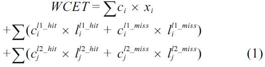
The equation above defines that the WCET is the maximum sum of the cost for each basic block and the cost of the CRD. The cost of each basic block is the scheduled latency (i.e., ci) multiplied by the number of execution counts (i.e., xi) of that basic block; and the cost of the CRD is the sum of the hit and miss latency of each cache line block (i.e.,
respectively for an L1 cache and
respectively for an L2 cache) multiplied by the number of cache line block hits (i.e.,

for an L1 cache and

for an L2 cache) and misses (i.e.,

for an L1 cache and

for an L2 cache), respectively. The symbols used in this paper are explained in Table 1. More detailed information on IPET can be found at [4].
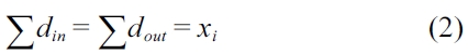
Equation (2) models the structural constraints of this program, which can be derived from the control flow graph (CFG) of the program.
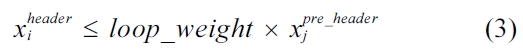
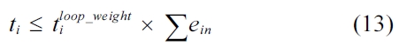
Equation (3) bounds the execution count of a loop header block. Basically, the execution count of a preheader block timed by the weight of that loop should provide the upper bound for the execution count of this loop header block.
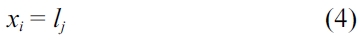
Equation (4) describes the fact that the execution counts of a basic block should be equal to the execution counts of the L1 cache line block holding this basic block.
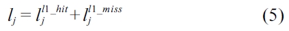
Equation (5) states that the sum of L1 cache hits and misses for a cache line block
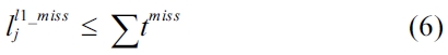
Equation (6) gives a tighter bound of the number of L1 cache misses for a cache line block

will be detailed in Section III-C.
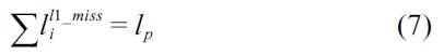
Equation (7) is based on the fact that the number of execution counts of a lower level cache line should be equal to the number of execution counts of cache misses from its corresponding upper cache line.
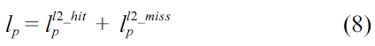
Equation (8) breaks the execution counts of a lower level cache line (i.e., an L2 cache line) into two parts, including the number of cache hits and the number of
[Table 1.] Symbols used in this paper and their description

Symbols used in this paper and their description
cache misses. Similarly to Equation (5), this equation also gives the first upper bound for the number of misses from L2 cache lines.
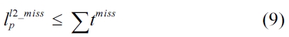
Equation (9) gives another bound regarding the number of misses for a cache line block, in which
will be further bounded in our address flow analysis. It should be noted that it is possible for users to provide more data flow analysis constraints to help reduce the number of infeasible paths, which may make the ILP solver derive even tighter WCET analysis results.
A program’s WCET is determined by the execution time of the code and the CRD caused by loading the instructions and its data to the processor. In our model, thanks to the help of a compiler and a statically-scheduled architecture based on very long instruction word (VLIW) [16], the execution time of each instruction can be statically derived from its static scheduling. However, the CRD is still subject to the dynamic program behavior in terms of the instruction and data memory access patterns and the history of accesses, as well as the actual cache architecture (i.e., cache set associativity, replacement policy, etc.). In a multicore processor with a shared cache, the CRD is also dependent on the memory access behaviors of other concurrent threads that may access the same cache. Motivated by this observation, we start with the address flow analysis and introduce the AFG to unify instruction and data cache timing analysis and to help transform the CRD into an ILP problem that can be automatically solved in a reasonable amount of time.
An AFG,
An edge
From the AFG’s point of view, the execution of a program can be viewed as running a sequence of addresses loaded from the memory to the processor. This sequence is subject to the control flow of a program to ensure correct semantics. Therefore, the control flow graph can be directly used to represent the AFG for instruction accesses. However, we will analyze the limitation of simply using the CFG to represent the AFG when considering data caches in Section III-B-4, which necessitates the concept of AFG for the timing analysis of unified caches that are common for last-level caches.
In the rest of this section, we will begin with the AFG based analysis for a simple direct-mapped instruction cache and then extend to more complicated cache structures.
1) AFG for Direct-Mapped Instruction Caches
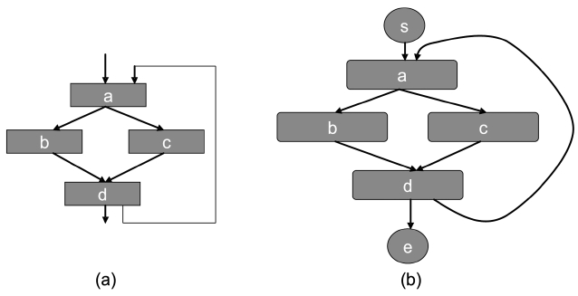
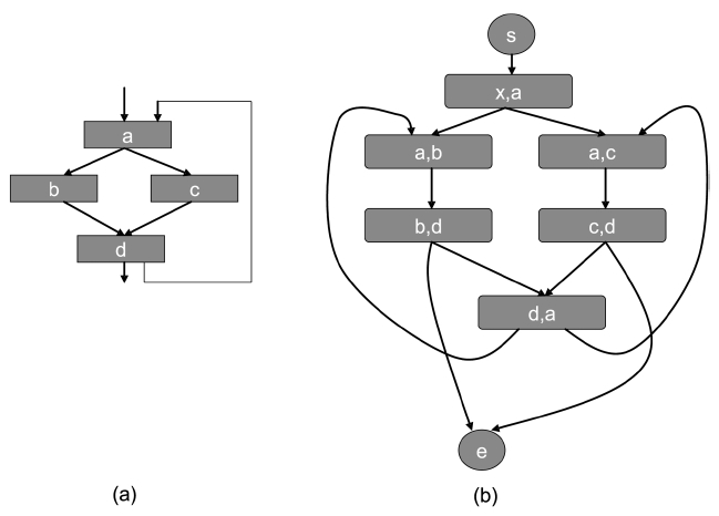
We assume a virtually-addressed cache. After compilation and linking, the virtual address of each instruction is known. Given a cache, each instruction can be mapped to a particular cache line for a direct-mapped cache or to a particular cache set for a set-associative cache in general. Assume that we have a CFG as shown in Fig. 2a, which has 4 instructions,
From this example, it can be seen that in a directmapped cache, the state is solely determined by the instructions accessed. Thus, each address (or instruction) forms a vertex in the AFG.
2) AFG for Set-Associative Instruction Caches
Now let us consider a more complicated and generic scenario, i.e., a set-associative cache. The contents of a set-associative cache consist of the history of cache
accesses and the current access. Therefore, for an AFG to correctly represent the address flow of a set-associative cache, the vertex in the AFG must be able to:
· Memorize the history cache accesses;
· Represent the change caused by the current cache access;
· Derive the next possible cache access without violating program semantics.
This can be achieved by using a tuple, called a cache line state (or a cache set state),
In Fig. 3a, the same assumption is made as the case of a direct-mapped cache, except that the cache is now a 2- way set-associative. Assume that the initial state of the cache set
3) AFG for Instruction Caches Shared by Multiple Threads
A more complicated scenario involves two or more threads running simultaneously on a multicore access to a shared cache such as an L2 cache. Then, the abovementioned cache state
Motivated by this, assuming we have
4) AFG for Data Caches
Now, let us take data caches into consideration. In contrast to instructions in a program, data cache WCET analysis typically has difficulty in acquiring the address information for each load/store instruction. Furthermore, what makes it even worse is that even if the data address of each load/store is known, a 1-to-
To determine the data address for general-purpose applications such as programs with pointers and dynamic memory allocation is a very challenging task. Fortunately, hard real-time applications typically restrict the use of those features such as dynamic memory allocation; therefore, it is not uncommon to assume that the data access addresses are statically known for timing analysis in the domain of hard real-time systems, which is also the assumption used in this paper (it should be noted that the focus of this paper is not to tackle how to statically generate addresses for data cache timing analysis, which is orthogonal to our research. Instead, a contribution of this paper is to use AFGs to represent the data and/or instruction addresses, based on which our method can derive the WCET for multicore processors). In addition, we assume for programs with loops, the maximum number of loop iterations is known, which can be either obtained by static analysis or annotation.
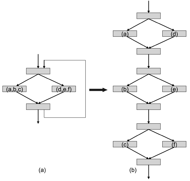
Based on the assumption that the data addresses for each load/store and the correct access sequences can be known statically, we propose to expand load/store operations to create the AFG. The idea is to unroll the loop so that the data address accessed by each instance of a load/ store operation in each loop iteration is represented as an individual vertex in an AFG. For nested loops, our approach starts from the innermost loop to conduct load/store
expansion. Each expansion of the loop needs to remove the back-edge of the expanded loop, while maintaining all the other edges to keep the control flow information. After load/store expansion, each data access can be uniquely represented by an address; therefore, the AFG for a data cache can be constructed in the same way as that for an instruction cache. It should be noted that currently we focus on loop index based accesses; however, the approach can also be extended to any accesses sequence as long as the correct address sequence can be statically obtained. Moreover, the AFG for set-associative data caches and shared data caches can be similarly constructed by using the same principles for instruction caches as discussed in Section III-B-2 and Section III-B-3.
An example is shown in Fig. 4 to illustrate our approach. For simplicity, suppose that we have a loop with three iterations and two load instructions. One load instruction accesses addresses
It is worthy to note that the instruction accesses and data accesses are treated in the same way in an AFG, for which only the addresses of instruction or data accesses matter. Therefore, our discussion on the AFG for setassociative caches in Section III-B-2 and AFG for shared instruction caches in Section III-B-3 can be directly applied to the data accesses. However, a major difference between a data access and an instruction access is that inside a loop, the same instruction and thus the same address is accessed for different loop iterations; while for data accesses, the same instruction at different loop iterations may access different memory addresses. This problem can be solved by using the load/store expansion as mentioned above. Therefore, after building the AFT after using load/store expansion, the analysis for the data cache or shared data cache is not different from the instruction cache or the shared instruction cache as previously discussed.
>
C. Implementation of the AFG
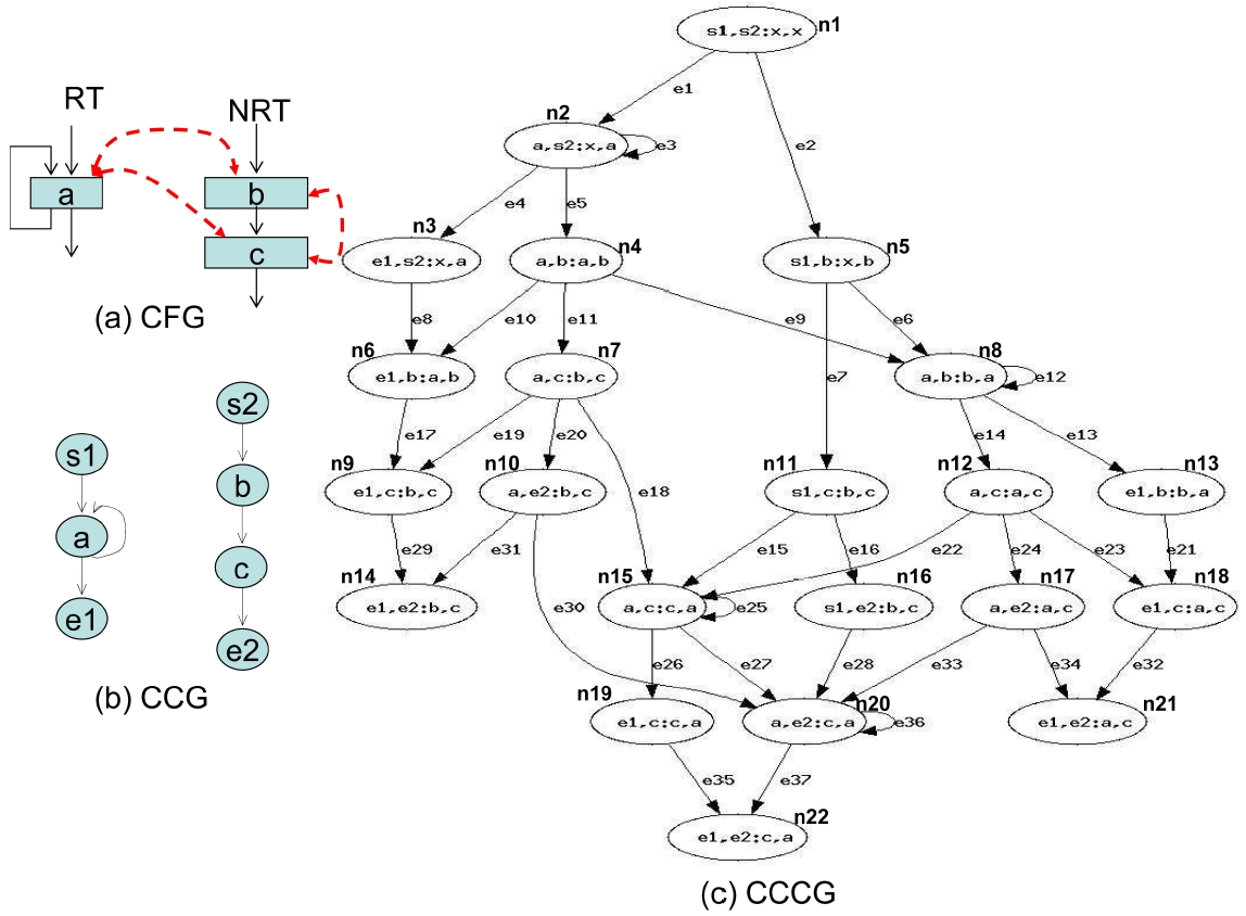
Section III-B discusses the definition of an AFG and its application in different cache structures. In this section we propose to use a combined cache conflict graph (CCCG) to realize the AFG for our assumed architecture, which can handle instruction as well as data caches, direct-mapped as well as set-associative caches, interthread shared cache and multi-level cache hierarchies.
The CCCG can be built upon the cache conflict graph (CCG) [4,5] of each concurrent thread. The CCG was first proposed by Li and Malik [4] and Li et al. [5] to bound worst-case instruction and/or data cache misses for single-core processors. A CCG is basically a projection of a control flow graph for a given thread on a cache set, which contains a set of nodes and edges. In a CCG, each node corresponds to a cache set, and each edge represents a legal path in the CFG between two nodes. A CCG is constructed for every cache set containing two or more conflicting memory object accesses (i.e., instructions or data addresses mapped to the same cache set). A CCG contains a start node ‘s’, an end note ‘e’, and a node ‘
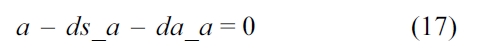
In a CCCG, each vertex is denoted by a tuple
1) Build the CCCG
For illustration purposes, we assume that we have 2 threads (i.e.,
[Algorithm 1-1] The construction of a CCCG
The construction of a CCCG
where
Algorithm 1 takes the initialized state t and starts walking from the thread
2) Bounding Cache Hits
The sum of all the entry edges should equal to 1, as shown in Equation (10). An entry edge is an edge in a CCCG that starts the entry block in a CCG. Specifically, this edge has a source state containing the start entry and its destination state has an entry other than the start entry.
Each CCCG is subject to its own structural constraints as shown in Equation (11). The sum of in-flow edges equals the sum of out-flow edges, which equals the number of execution counts for the current state. However, in a CCCG, each cache line block may sit in a different

in Inequality (13) is a constant.
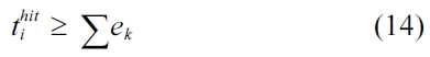
The cache hit bound is calculated by Inequality (14), where
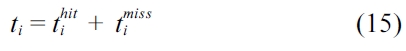
Equation (15) links the bounded cache hits and misses to the total number of execution counts of the state
The constraints from Equations and Inequalities (2)- (15), in conjunction with the objective function (1) can be solved by using an lLP solver. The result of the objective function will be the WCET
Fig. 5 gives an example to illustrate how to apply the CCCG to WCET analysis. For simplicity, assume there are two threads, a real-time thread (RT) and a non-real-
time thread (NRT) (It should be noted that the CCCG can be applied to multiple RTs as well). While the RT has only one instruction
The following objective function below is derived from Equation (1).
Structural constraints are derived from Equation (2). First, we construct the structural constraints for the RT. In the following equations,
starts from the instruction
Also, we can construct structural constraints for the NRT as the follows.
>
C. Functionality Constraints
For each thread, we assume that each of them executes only once.
We also assume that the loop in the RT thread executes no more than 10 iterations, which is based on Equation (3).
Cache constraints are obtained from Fig. 5c.
1) Connection Constraints
The following equation describes the constraints, i.e., the sum of instruction
2) CCCG Entry Edge Constraints
The RT thread executes only once; thus we have the following equation, which is based on Equation (10).
Similarly, the NRT thread also executes only once, leading to the following equation.
3) CCCG Node Constraints
The sum of all the nodes that execute instruction

Similarly, the sum of all the nodes that execute instruction
Also, the sum of all the nodes that execute instruction

4) Hit Edge Constraints
The following equations are derived from Equation (13).


5) CCCG Hit Bound
The total cache hits of instruction
6) Put Them All Together
Fig. 6 shows the WCET path for the example. The final result from ILP (i.e., the WCET) is 208, which can be derived from Equation (37).

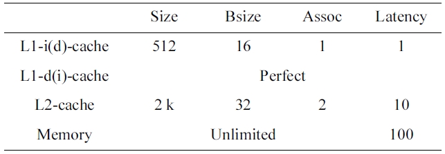
It should be noted that in this paper, we assume a timepredictable bus and memory system [17], so that we can focus on studying the timing analysis of the shared caches for multicore processors. In our experiments, we use a cycle-accurate simulator based on SuperESCalar (SESC) simulator to simulate a dual-core processor with either a shared L2 instruction or data cache. The memory hierarchy of the dual-core processor is specified in Table 2. The LP analyzer is implemented by incorporating a commercial ILP solver, CPLEX [18] to handle the linear programming analysis, which generates the worst-case number of misses for both the L1 instruction and data caches and the L2 cache, as well as the WCET.
In the experiments, we chose 10 real-time benchmarks from Malardalen WCET benchmarks [19], and 2 mediabench applications from Mediabench [20]. Then, each benchmark runs concurrently on the dual-core processor with a benchmark called crc, which is randomly selected from Malardalen WCET benchmark suite [19].
>
A. Instruction Cache Timing Analysis Results
To evaluate the effectiveness of the proposed approach,
[Table 2.] Cache configuration of the base dual-core chip

Cache configuration of the base dual-core chip
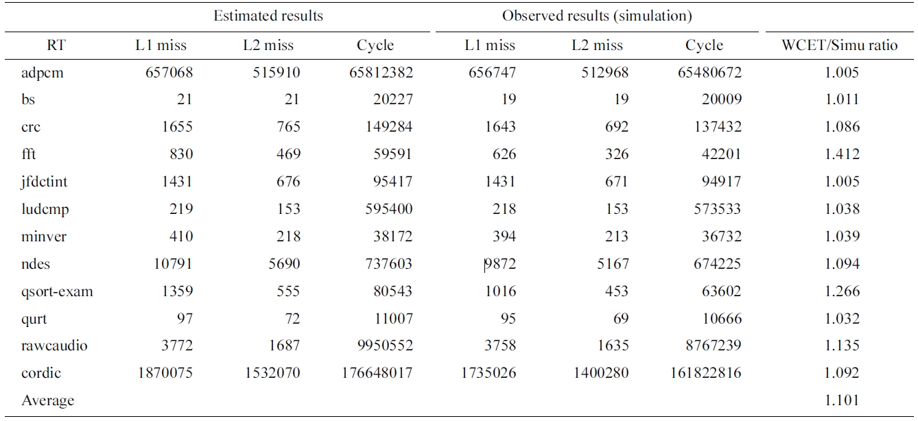
we first study the timing analysis for a dual-core with a shared instruction cache. Table 3 compares the estimated and observed (through simulation) number of L1 misses, number of L2 misses, and execution cycles. The last column gives the ratio of the estimated WCET by our approach to the observed WCET through simulation. As can be seen in Table 3, for a number of benchmarks such as adpcm and jfdctint, the proposed approach can obtain a very tight upper bound of execution cycles, which are within 1% of the observed WCET. On average, the estimated WCET of our approach is 10.1% more than the observed WCET through simulation, which is very accurate considering all possible inter-core cache interferences. Also, we observe that our approach can accurately estimate the worst-case number of L1 and L2 cache misses, which are not too far away from the observed worst-case results.
However, it should be noted that although our approach can achieve a tight bound for most of the benchmarks, the worst-case performance of some benchmarks is still overestimated. In particular, we notice that the estimated WCETs of fft, qsort-exam are 1.412, 1.266 times more than the simulated results, respectively. One of the major reasons for this overestimation is the intensive ifthen- else used in the loops in these programs. In both programs, if-then-else in loops typically make the programs execute one of the branches (e.g., a then branch) consecutively and then switch to the other branch (e.g., a else branch) stay that way for later iterations. This will certainly improve the cache hit ratio since the instructions in either branch are consecutively placed in the cache memory, which can be reused and thus lead to more cache hits. However, in the ILP’s semantics, the execution of an if-then-else in a loop is most likely inter-

Comparing estimated and simlated worst-case L1, L2 misses and execution cycles for the shared instruction cache
interpreted alternatively (e.g., executing one path and then the other path without repeating each path more than once). This is because such an execution on alternative paths can result in a theoretical worst case, which however may not happen at runtime. It is worthy to note that providing further information such as data flow or infeasible paths can help to reduce the overestimation if there is any.
>
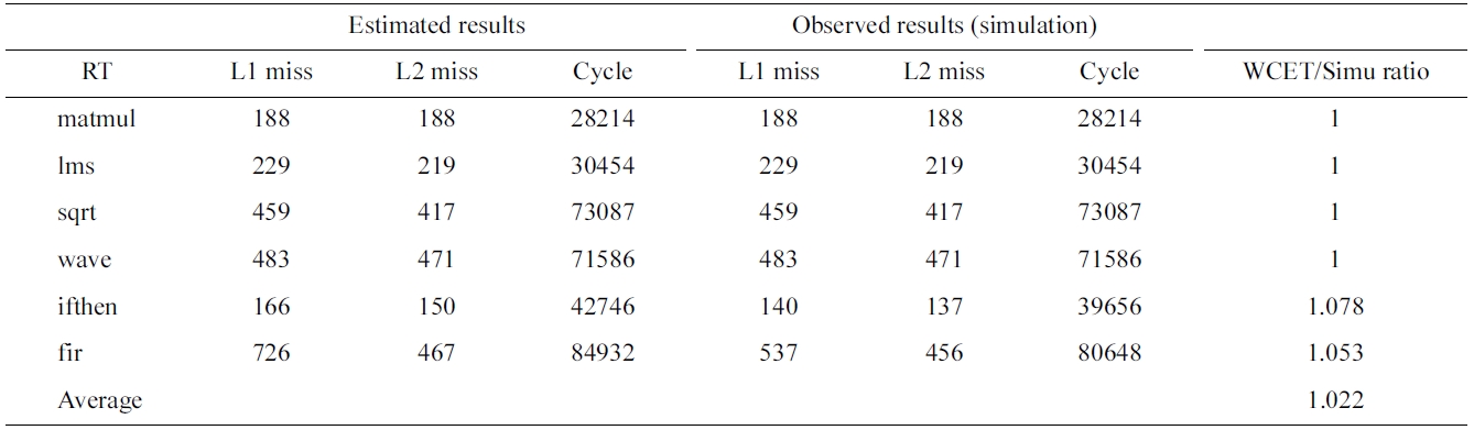
B. Data Cache Timing Analysis Results
As a proof-of-concept study to verify the effectiveness of the proposed load/store expansion approach, we choose six benchmarks whose data access addresses can be statically computed from Malardalen WCET benchmarks [19]. Table 4 compares the estimated and simulated number of L1 misses, number of L2 misses, and execution cycles for the shared data cache of the simulated dual-core. The last column provides the ratio of the estimated WCET to the observed WCET through simulation. As can be seen in Table 4, the proposed approach can precisely obtain the theoretical WCET on four benchmarks
This paper presents a novel and unified approach to bounding the worst-case performance of shared instruc-

Comparing estimated and simlated worst-case L1, L2 misses and execution cycles for the shared data cache
tion and data caches for multicore processors. While traditional control flow graph based analysis is useful for instruction cache analysis, it is not effective for analyzing data caches, which are important components of multicore chips. To address this problem, we propose to use address flow graphs to model all the possible inter-thread cache conflicts, including both instruction and data accesses, based on which our method can accurately calculate the worst-case inter-thread cache interferences and derive the WCET. We also describe a general method to use combined cache conflict graphs to automatically implement AFGs for set-associative caches shared by multiple threads.
Our experiments indicate that the proposed approach can accurately compute the worst-case performance for real-time threads running on a dual-core processor with a shared L2 cache (either to store instructions or data). Compared to the observed WCET, the estimated WCET is 10.1% larger on average, and can be as low as 1% or less for a number of benchmarks for shared instruction cache analysis. For shared data cache analysis, the estimated WCET is within 2.2% on average compared to the observed WCET by simulation.
In our future work, we would like to conduct unified cache timing analysis on large benchmarks and more cores. Also, we are working on reducing the number of states modeled by CCCGs without affecting the safety and accuracy of analysis. For example, numerous impossible states can be removed by firstly eliminating the infeasible paths on all the concurrent tasks.