In this paper we present a framework for a novel kind of context-aware preference query composition whereby queries for the Preference SQL system are created. We choose a commercial e-business platform for outdoor activities as a use case and develop a context model for this domain within our framework. The suggested model considers explicit user input, domain-specific knowledge, contextual knowledge and location-based sensor data in a comprehensive approach. Aside from the theoretical background of preferences, the optimization of preference queries and our novel generator based model we give special attention to the aspects of the implementation and the practical experiences. We provide a sketch of the implementation and summarize our user studies which have been done in a joint project with an industrial partner.
I. INTRODUCTION AND RELATED WORK
Clearly, this state of affairs is non-satisfactory for both the users and the owners of the portals. In new tourist portals (like presented in [5]), preferences allow for semantically richer queries which define a strict partial order on the items available for the purpose of selecting
only the best items available, yielding a higher customer satisfaction.
In domains like tourism, the notion of preferences varies between users and strongly depends on users’ situations. Hence, recent models of context-aware preferences emerged [6-9], which are taking into account factors like users’ personalities, situation parameters (e.g., location, time, season, weather), or even options of users’ acquaintances. [6] introduces CareDB, which provides scalable personalized location-based services to users based on their preferences and the current surrounding context. In particular, it deals with the problem that some contextual values may be very expensive to compute. [8] suggests a context-model for preference queries, where context is represented by a variant of description logic.
[9] suggests a discrete context model and introduces profile trees as a data structure for the context resolution problem, hence retrieving the most appropriate preferences depending on context. Similarly, [7] suggests a model for a contextual preference selection based on the idea of a situation hierarchy. These models can be seen as top-down approaches in contrast to our constructive bottom- up model. In our approach all preferences are generated dynamically instead of performing a look-up in a set of predefined preferences.
There is the open challenge to create a comprehensive framework to derive preferences from context. In this paper, we meet this challenge by presenting an approach for the context-aware preference composition, which 1) produces inductively structured preference queries that are intuitive such that they can be verified by domain experts, 2) allows for easy adaption of the composition process for the specific application domain, and 3) covers the entire path from the descriptive application model to the operational preference query language.
Throughout the paper we refer to the following example from the domain of hiking tour recommendations which informally demonstrates the lines of reasoning about context-aware preferences of domain experts (like touristic companies). Thereby, we want to model: social network (recommendations from friends), history (already visited regions by the user), and external knowledge sources (weather services, like the snow line and the altitude- dependent temperature).
EXAMPLE 1 (Running use case). Consider John, who is planning a hiking tour in the touristic region of the Bavarian Alps. Last year, he was in the “Tannheim Mountains” and a friend of his made a tour in “Walser Valley” which he was very excited about. Since John now wants to see something new, he wants to avoid regions he has already visited. At the same time, he trusts his friends and thus prefers regions recommended by friends.
As he is not very experienced, he only specifies duration for the tour, while he relies on the recommender for the ascent and length. John prefers not to hike in the snow; hence, only mountain peaks below the current snow line are preferable for him. Because it is a sunny day, the temperatures in low altitudes are too high, so the tour should mainly take place in a convenient altitude range.
John looks out for an online portal which picks out a hiking tour from a large database that perfectly matches the preferences formulated above. In case there are no “perfect tours” he accepts compromises, e.g., tours whose altitude exceeds the snow line a little bit.
The remainder of the paper is structured as follows: Section II informally presents the preference model used in this paper. Thereafter, Section III describes our context- aware preference generation process. Section IV shows how the generated preference queries can be evaluated using Preference SQL. Section V provides a conceptual view of the entire system and its implementation. Finally, Section VI summarizes our claimed contributions and outlines further research directions.
Preference modeling has been in focus for some time, leading to diverse approaches [1,3,10]. We follow the preference model from [1], which directly maps preferences to relational algebra and declarative query languages. It is semantically rich, easy to handle and very flexible to represent user preferences which are ubiquitous in our life.
A
DEFINITION 1 (Preference selection, BMO-set).

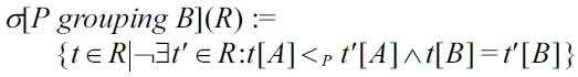

Preference selection offers a cooperative query answering behavior by automatic matchmaking: The BMO query result adapts to the quality of the data in the database, defeating the empty result effect and reducing the flooding effect by filtering off the worse results.
To specify a preference, a set of intuitive base preference constructors together with some complex preference constructors has been defined. Subsequently, we present some selected preference constructors used in this paper. More preference constructors as well as their formal definition can be found in [1,3].
1) Base Preference Constructors
Preferences defined on a single attribute are called
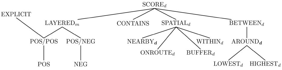
The SCORE
scores together. Such a real-world behavior can be modeled using the
We now explain some categorical sub-constructors of the SCORE
DEFINITION 2 (POS and NEG preference).
EXAMPLE 2 (Running use case). Reconsider Example 1 where John is planning a new hiking tour. Since John trusts his friends he wants to avoid regions he has already visited and therefore prefers regions recommended by his friends. Using the POS and NEG preference constructors from Definition 2 these preferences can be formulated as
P1 := POS(recommended, ‘yes’)
P2 := NEG(visited, ‘yes’)
where
Now, we present some preference constructors for continuous domains.
DEFINITION 3 (BETWEEN
The AROUND
DEFINITION 4 (AROUND
EXAMPLE 3 (Running use case). Continuing Example 1 John prefers a hiking tour with a duration of around 5 hours. Thereby, John accepts tours which take ±10% of the desired time, i.e., he uses d-parameter of 0.5 hours. Using the AROUND
P := AROUND0.5 (duration, 5)
Sometimes one prefers values
DEFINITION 5 (LESS_THANd, MORE_THANd).
a) The MORE_THANd (A, z) preference equals the BETWEENd (A, z, ∞ ) preference, i.e., the desired values are greater or equal to z.
b) LESS_THANd (A, z) is the dual preference to MORE_THANd (A, z) and equals BETWEENd (A, ?∞,z); i.e., the desired values are less or equal to z.
EXAMPLE 4 (Running use case). John does not prefer to hike in the snow, hence only mountain peaks below the current snow line of 2,400 m are preferable for him. This leads to a LESS_THAN
P := LESS_THAN200 (altitude, 2400)
2) Complex Preference Constructors
If the user wants to combine several preferences into more
DEFINITION 6 (Pareto preference).
P := P1 ?...? Pm = (A1 × ... × Am, The DEFINITION 7 (Prioritization preference). P := P1 & ... & Pm = (A1 × ... × Am, EXAMPLE 5 (Running use case). John prefers a hiking tour with a PJohn := AROUND0.5 (duration, 5) & (POS(recommended, ‘yes’) ? LESS_TRANda(altitude, 2400)) The variable For the rest of this paper we also need the notion of a preference term. DEFINITION 8 (Preference terms). A base preference P = (A, The semantically well-founded approach of this preference model is essential for the personalized preference term composition. As a unique feature this preference model allows multiple preferences on the same attribute without violating the strict partial order. Furthermore, the
III. CONTEXT-AWARE PREFERENCE GENERATION
Based on the preference framework presented in Section II we will now present our model for creating preference terms dependent on the context. This model depends on context-based triggers which are described by a discrete situation model with few states. Compared to continuous models, such models are particularly useful when communicating with domain experts as the small number of states makes it possible to systematically consider all combinations of context states and therefore guarantee that the system behaves in the desired way for all possible context values. For example, concerning the weather, it is intuitive to distinguish between “good” and “bad”. For our domain of a hiking tour recommender we introduced the states: “good”, “bad” and “warning”. Whereas, “bad” implies less convenient outdoor activities, the state “warning” discourages activities like hiking because of safety reasons. Dependent on the context (time of year, region) alternatives like city tours or visiting the spa could be suggested.
>
A. A Constructive Approach for Preference Generation
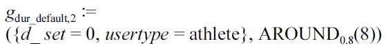
According to our running use case of a hiking tour rec-ommender we have three different kinds of influences for the preference generation: The user input from the search mask, the user profile from the database and the contextual information from external knowledge sources. In the following we describe how they interact in our model. As described in Example 1, the weather conditions imply certain preferences. However, weather warnings do not mean that the user input is overridden. The rough concept of the preference composition always follows this prioritization- schema, where each <...>-part is called the
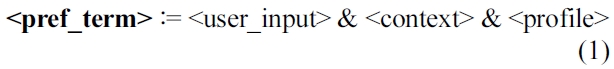
The
The gravity of the external influences depends on the user: a well specified user input, i.e., all fields of a search mask are filled out, implies that the context and the profile have only minor influence to the generated preference. If a “lazy” user leaves all fields blank, a “default request” based on the context and the profile will be generated.
In the following, the components of (1) are stepwise filled with preferences. This procedure underlines our
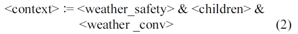
In the
In the
The components
EXAMPLE 6 (Running use case). Consider the tourist John who has only specified a duration of 5 hours for his tour. In our tour recommender this preference is modeled with the AROUND-constructor. Thereby, we assume a tolerance of 10% which leads to a
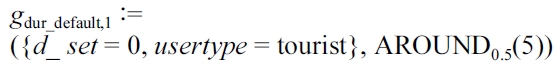
Depending on empirical values like average speed and condition of his user type (e.g., “tourist” or “athlete”), the system selects defaults for length and ascent according to the duration. Assume that the role of John, e.g., tourist, implies default values of 12 km for the length and 600 m for the ascent, both with a
The Pareto-composition of these preferences is based on the assumption that the attributes of length and ascent are of equal importance for the user. This ordering may depend on the user type, e.g., an athletic user is focused on the ascent of the tour whereas an inexperienced tourist is more confident to the duration, i.e., the preferences in our use-case also depend on the “tourist role”, which is investigated in [14].
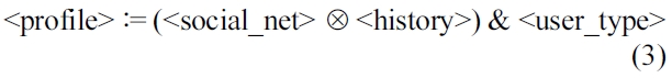
The social network and the history in (3) are Paretocomposed to take care of both aspects. In the following example we will show how conflicting preferences can be handled.
EXAMPLE 7 (Running use case). We assume the attributes
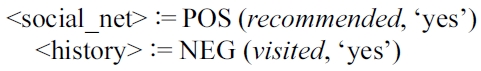
According to the Pareto composition
The preference model from Section II gives us the freedom for this component-based model, where preferences with oppositional influences have a meaningful semantic interpretation in our preference model.
To fill the
The generation of preferences in our approach is context- aware in two regards: 1) preferences in the components are triggered by a discretized context, and 2) parameters of these preferences can change with the continuous context.
By this breakdown the model is kept clear. Whereas in the “discretized world” the rough structure of the preference term is decided, the “continuous world” influences the fine structure of the preference term. Thus, it is easy to see how the configuration of the recommender changes the final output.
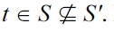
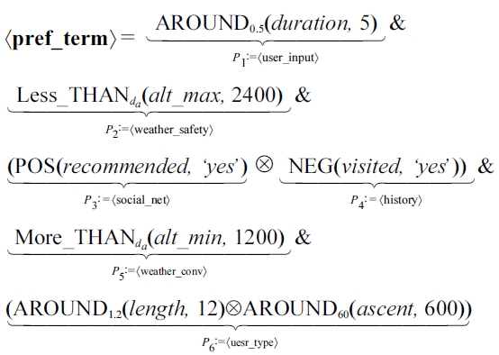
DEFINITION 9 (Context variables, [current] situation).
vi : Ω → Vi for i ∈ {1, ...,n} =: I
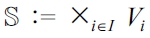

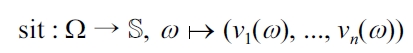
{vi = α} := V1 × ... × Vi-1 × {α} × Vi+1 × ... ×Vn.
We illustrate the concept of context variables in the following example.
EXAMPLE 8 (Running use case). To describe the current weather state of the hiking region selected by the user input, we introduce a context variable
By
With the context variables we will trigger the rough structure of the
DEFINITION 10 (

is the set of
holds.
EXAMPLE 9 (

The term LESS_THANda(
The interplay of the rough and the fine structure of preference generation is done by the
DEFINITION 11 (Context-aware generator).
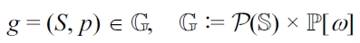
EXAMPLE 10 (Running use case). To realize the components
gch := ({children = yes},POS(difficulty, ’easy’))

gws,2 := ({weather = bad}, LESS_THANda (alt_max, min(snowline(ω), 1500)))
gws,3 := ({weather = wrn}, POS(activity, ’CityTrail’) & LESS_THANda(alt_max, min(snowline(ω), 1500)))
Thereby wrn is short for warning. Whereas

the generators
>
C. Constructing Preference Terms from Generators
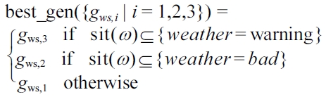
Now we have components and associated sets of generators. The next step is to select the active generators and to create a preference term from them. To this end we have to specify how the preferences of the generators shall be Pareto-composed or prioritized if there is more than one generator associated with a component.
Assume an ordering of the generators representing the

we realize this by a function
where smaller values stand for a higher importance. The
In order to transform a set of generators to a preference term, first, the active generators are determined (Definition 12). With Definition 13 we realize the principle that preferences created by more important generators are prioritized, and Pareto-composed if the according generators are equally important.
DEFINITION 12 (Restriction to situation, active generators). Consider a set of generators


G|s := {(S, p) ∈ G | s ∈ S}
DEFINITION 13 (Preference generation).

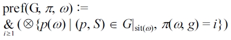
where ?{p1, ..., pn} := p1 ?...? pn and

qi := q1

The configuration of a component is described by the tuple (G, π).
Preference terms generated with the pref-function from Definition 13 - also known as
Hence, generators which are more specialized to the current situation are preferred to less specialized ones. This unveils a nice analogy to the “best matches only” principle, but now we look out for the
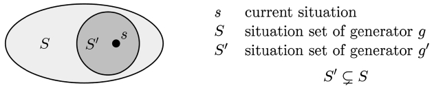
DEFINITION 14 (Best matching generators).

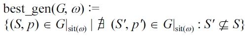
In Fig. 3, the situation sets of two generators are illustrated. The best_gen function applied to {
A similar concept also occurs in [9]. But since we use this concept only to
EXAMPLE 11 (Running use case). In Example 10 using Definition 14 only one generator is in the set best_ gen({

for
>
D. The Context Model in the Use Case
To apply the context model to Example 1 from the introduction we are still missing some definitions. We have generator sets for all the components of the
We exemplify the formal notation of the generators for
EXAMPLE 12 (Running use case). Assume the context variable

the
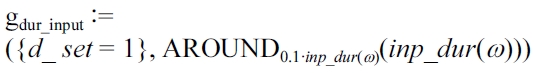
For the
In an analogous manner we define generators for ascent and length. These definitions produce the desired user input and the user type dependent input.
Thus, the concept of generators is “reused” for this component: By allowing that the input from the search mask is also stored in
In the following example we subsume our results and demonstrate how the entire preference term is composed.
EXAMPLE 13 (Running use case). According to the previous examples and the assumption that convenient weather conditions imply a minimal altitude (attribute
Thereby we use the rough structure from Eqs. (l)-(3),
With this we have defined a model which is applicable for our problem of designing a hiking tour recommender. But we still have one drawback with the assumption that all the external information in
For example, we assumed we have access to the complete weather forecast to determine the values of our context variables. However, what if the user did not specify a region for the activity or too big of a region to obtain a reliable weather forecast? Or what shall the recommender do if the weather service is unavailable? This can be modeled by replacing the current situation
by a set of current situations
with
Ω0 ⊆ Ω
where all weather states are contained, formally {
for all
IV. CONTEXT-AWARE PREFERENCE QUERY EVALUATION
The complex preference terms generated in Section III must be evaluated efficiently to retrieve the best-matching objects for the user. Therefore, we discuss in this section the Preference SQL system which provides a query language for evaluating preference queries. Moreover, we present some optimization techniques for preference optimization and present some practical performance benchmarks.
1) Preference SQL Syntax:
Preference terms can be transformed into Preference SQL, an extension of standard SQL for preference query evaluation on database systems, cp., [11].
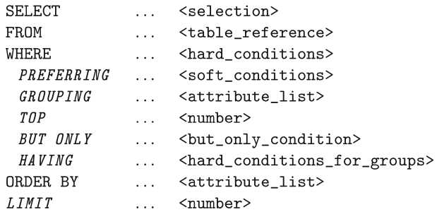
Syntactically, Preference SQL extends the SELECT statement of SQL by an optional PREFERRING clause. A preference query selects all best matching tuples, i.e., tuples that are not dominated by other tuples. The preference SQL currently supports most of the SQL-92 standard as well as many base and complex preference constructors. For a full overview we refer to [1,3,11]. For our goals, a Preference SQL query block has the following schematic design:
The keywords SELECT, FROM, WHERE, and ORDER BY are treated as the standard SQL query keywords. The PREFERRING clause specifies a preference by means of the preference constructors given in Section II and [11]. GROUPING allows a grouped preference selection, cp., Definition 1. Additionally, GROUPING contains the GROUP BY functionality as in the standard SQL if aggregate functions (such as sum(...), count(...), etc.) occur. HAVING allows for hard conditions for groups as in the standard SQL. Further keywords such as BUT ONLY, TOP and LIMIT are provided to modify the preference evaluation. BUT ONLY is used for the definition of post-filters, and TOP and LIMIT to regulate the size of the result set. After specifying a preference it is evaluated on the result of the hard conditions stated in the WHERE clause, return-ing the BMO-set. Empty results can only occur if the WHERE clause returns an empty result. For more details we refer to [11] and [16].
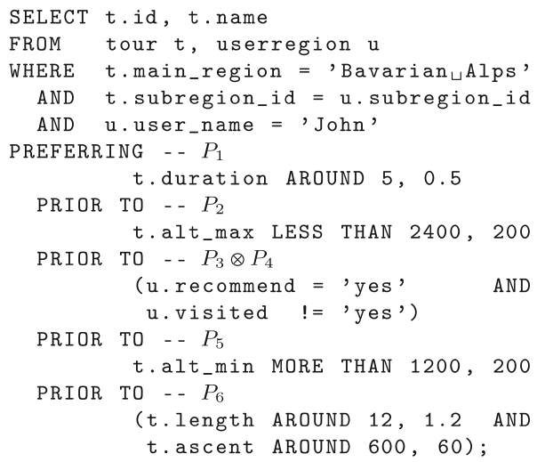
The final preference term from Example 13, e.g., can be formulated in Preference SQL as demonstrated in Fig. 5.
A Prioritization is expressed using PRIOR TO, whereas AND in the PREFERRING clause denotes a Pareto preference. The preference constructors AROUND, LESS THAN and MORE THAN are already known from Section II and III. Note that the second argument of these preference constructors denotes the
The query is executed on a productive tour database provided by Alpstein Tourismus GmbH (http://www.alpstein- tourismus.com). It returns all hiking tours in the Bavarian Alps which correlated best with the preference term from Example 13. All hiking tours are stored in the relation tour. There is a connection with the relation userregion, because it holds personalized information about recommendations and visited tours, cp., Example 7.
2) Preference SQL System Architecture:
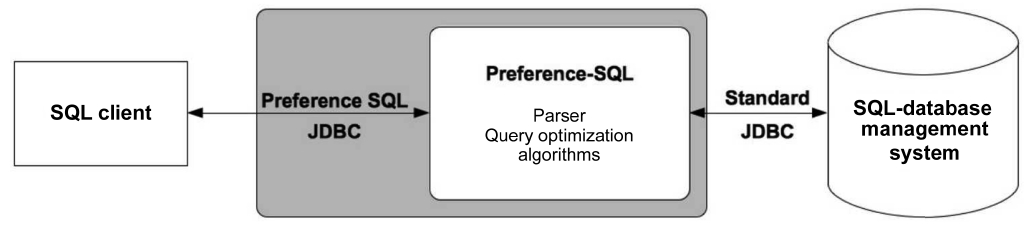
While the first prototype [17] used query rewriting to
standard SQL, the current implementation of Preference SQL (since 2005) is a middleware component between the client and database which performs the algebraic and cost-based optimization of preference query evaluation, (Fig. 6).
The “top of the database” approach allows a seamless, flexible and efficient integration with standard SQL back-end systems using a Preference SQL Java database connectivity (JDBC) Driver. This enables the client application to submit Preference SQL queries through familiar SQL clients. The Preference SQL middleware parses the query and performs preference query optimization as subsequently described. Those parts of an optimized query execution plan, which directly correspond to SQL- 92, are handed over to the attached SQL database system for evaluation. The (grouped) preference selection operator together with novel algebraic and cost-based query optimization methods are dealt within the Preference SQL middleware.
This trend is strengthened by [18], which even suggests implementing numerical preferences tightly in the relational database engine. According to [2] Preference SQL is currently the only comprehensive approach which implements a general preference query model.
>
B. Optimization of Preference Queries
A first view on the query in Fig. 5 leads to the assumption that the evaluation of this query on a database system is very inefficient. Executing such queries on large data sets makes an optimized execution necessary in order to maintain small runtimes. For this, Preference SQL implements the accumulated vast query optimization knowhow from relational databases as well as additional optimization techniques to cope with the preference selection operator for complex strict partial order preferences. Basically, in its current version a Preference SQL query is processed as follows:
1) The query is parsed and transformed into an initial operator tree annotated by preference relational algebra, which comprises classical relational algebra plus the preference selection operator [3].
2) Then heuristics for the algebraic operator tree transformation are applied. For this purpose, the familiar principles known from standard relational databases had to be augmented by new transformation laws for preference relational algebra (see [10,19,20] for details).
3) For efficient evaluation of the preference selection operator in our middleware, special efficient algorithms had to be implemented. For instance, for Pareto/skyline queries this repertoire includes the Hexagon algorithm [21] and LESS [22]. The algorithm selection is guided by a cost-based query execution model.
4) Likewise, guided by a cost-based model, the preference query optimizer determines suitable sub-trees of the final optimized operator tree for offloading them to the back-end SQL system. Those sub-trees are re-translated into SQL and sent via JDBC to the attached back-end afterwards [11].
5) The entire result of the query is assembled in our middleware and returned to the requesting client by the JDBC driver of the Preference SQL.
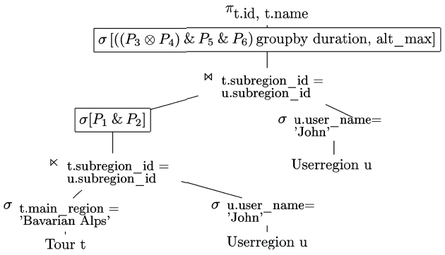
For example, the Preference SQL rule based query optimizer transforms the query from Fig. 5 into the operator tree depicted in Fig. 7.
The optimizer applies among well-known optimization rules the law
>
C. Practical Performance Tests
We now present some practical runtime benchmarks for the evaluation of context-aware preference queries.
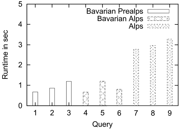
In our benchmarks the Preference SQL operates as a Java framework on top of a PostgreSQL 8.3 database. It stores the already mentioned real-world database of Alpstein Tourismus GmbH. The relations tour and userregion used in this paper contain approximately 48,000 rows and 200 rows, respectively. We build groups of three queries each with a specified
Query 4 corresponds to the preference query used in this paper, cp., Fig. 5. It can be evaluated in less than 1 second. The hard selection on the main region of the Bavarian Alps as well as the early computation of the
Query 7 is similar to Query 1. However, the basic set (about 16,000 tuples) is changed because of a different main region, namely the complete Alps. The runtime is about 3 seconds, which is fast enough for context-aware recommender applications, e.g., in the domain of hiking tours.
The evaluated queries are only a small selection of the queries occurring in our use case, but they are representative for our performance benchmarks. The runtime of these queries show that our approach of a context-aware preference query composition is not only intuitive but
also very efficient in computation of results on a productive database.
V. IMPLEMENTATION OF THE MODEL IN AN INDUSTRIAL PROJECT
In the previous sections we have described the theoretical foundations of our context model and the practical experiences with it according to our running use case from the introduction. In this section we describe our experiences with the context-model while implementing it in a joint project together with our industrial partner Alpstein Tourismus GmbH.
We present a sketch of the implementation of the context- model itself and also the entire system, including interfaces to the database and the backend for the domain experts. They are responsible for the content of the context- model, i.e., the preferences and the associated situation sets, organized in the context-aware generators. For example it is the task of the domain expert to adjust default values for length, duration and ascent for the different user types. It is also their task to define the contextvariables which span the situation set.
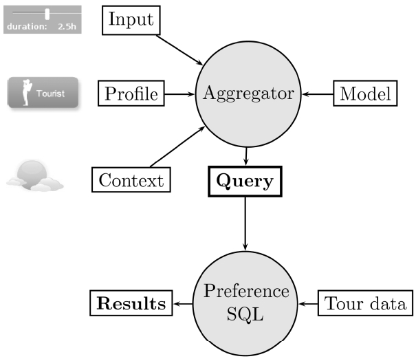
The implementation is mainly sub-divided in two parts: the first part is the generation of the query. To this end the input and the model must be brought together. We call the application performing this task the
The front-end for the user, where the user input is taken from. The input form is shown in Fig. 9. There the user has to select a user type (unless he is not a registered user) and his preferred values for length, ascent and duration.
If the user is registered for the portal, his user type is taken from the profile instead of the input form. There is also additional information in the profile, e.g., recommendations from the social network or the history of visited tours.
The information from external knowledge sensors is subsumed by the context.
The model content is stored in the database.
The generation of the query, based on the components above, is done in the aggregator.
The next part is the evaluation of the preference query. This is done using the Preference SQL and the tour database provided by our industrial partner. After the evaluation, the results are presented to the user. The architecture of the entire system is depicted in Fig. 10.
>
B. Sketch of Implementation of the Context Model
In the following we provide a brief description of the main concepts for the implementation of the context model.
There are some important classes:
Context, implementing a data structure for ω ∈ Ω from Definition 9. All the ω-dependant functions are fields of this class. Their type is arbitrary, but often numeric (e.g., snowline,...).
Situation, implementing the vi and
from Definition 9: Every context variable is a field of this class which may “null”. Thereby “null” expresses that the value of this variable is not known. Mathematically the “null” represents the set of all possible values for this context variable. Due to this, the Situation class represents not only single situations but also situation sets. As the context variables are discrete, the fields are usually of “enum” type, and sometimes they are also booleans for “yes/no” variables. The situation class contains methods to check if: - According to Definition 12: Check, if a situation is contained in the represented situation set.
- According to Definition 12: Check, if a situation is contained in the represented situation set.
- According to Definition 13: Check, if a situation set is strictly contained in another situation set.
Both methods obtain the fields of the situation class by the reflection techniques in Java, i.e., the methods do not have to be modified if new context variables are introduced.
Preference Term, implementing Definition 10. This is an abstract class for ω-dependant preference terms. It has concrete subclasses for complex preferences and base preferences, ω-dependant attributes are realized by function classes mapping a “Context”-object to a numerical domain.
Situated Generator, implementing Definition 11: This class has the attributes Situation and Preference Term; hence it implements our central concept of the context-aware generator. It contains also a numerical ranking field, which represents the π-function from Definition 13.
Finally a main class for the program, where the algorithm from Definition 13 is implemented, i.e., the entire preference term is generated.
The content of the model (i.e., the generators and the associated situations and preferences) is stored in a database via Hibernate; hence, Java objects representing the concrete model are created automatically.
Based on the implementation we completed some qualitative user studies presented in [5]. We will recapitulate and summarize the results in the following.
The technical criterion of the tests is the runtime; the user acceptance testing includes:
Session time of test subjects
Behavior: success, abort or iteration
Comments of test subjects
We compared the Faceted search without any context model, described in the introduction, with the preference search based on the context model, described in the running use case. Additionally, the results of the preference search have been analyzed by the domain experts from our industrial partner. The details of the evaluation can be found in [5]. The tour database contained approximately 48,000 tours.
In summary, we obtained the following results:
1) The run time of the generated Preference SQL queries never exceeded 5 seconds.
2) The session time of the preference search was about half of the session time with the Faceted search.
3) The test subjects expected “larger” result sets executing the preference search - due to the many preferences generated in the context-model, the result set was often quite small (<5 tours).
4) Empty results are still present in the preference search due to hard selections like geographical restrictions.
5) The flooding effect was never noticed executing the preference search. The result set mostly consists of 1-7 tours.
6) The average quality of the result set of the preference search was rated as 1.6 by domain experts - where 1 means “best” and 3 means “worst”.
In this paper we present a new approach to contextaware preference query composition which covers everything from context modeling to generating the preference query in a well known preference query language. Preferences, after being retrieved from a repository, are composed - on the fly - depending on context. The construction is performed by an algorithm which generates the bestsuited composition of context-dependent preferences per actual situation. The algorithm relies on a discrete context model, where preferences are associated to situation sets. Since the context model as well as the context-sensitive preferences have an explicit declarative description, domain experts may easily adapt or extend the model to meet their specific requirements without any changes to the generation algorithm.
By using discretization and context dependent functional mappings, we achieve an easy to understand system that is suitable for commercial applications. A running use case from the field of commercial e-business platforms for outdoor activities is used to motivate and illustrate the various steps in the process. The performance evaluation demonstrates that the answers for the generated queries can be computed efficiently on realistic data sets. Due to the BMO principle the trial and error behavior is replaced by a one-shot behavior which significantly reduces the session time at a high level of customer satisfaction. We have sketched an implementation which proved its value in a joint project with an industrial partner. The qualitative user studies underline the practical relevance of our work.
For future research we are working on further optimizing the queries using algebraic optimizations. Furthermore, we investigate preference modeling, especially the composition of complex preferences. In the use case presented in this paper we observed that in long chains of prioritization preferences containing Pareto preferences (cp., Fig. 5) the last occurring preferences of the term are often not decisive for the query result. In some cases, users rate the results as counterintuitive. In [23] we analyzed this effect in detail and suggested a new kind of Pareto preference as a remedy.