Biomass has become a major feedstock for bioenergy and other bio-based products because of its renewability and environmental benefits. Various researches have been done in the prediction of crucial characteristics of biomass, including the active utilization of spectroscopy data. Near infrared (NIR) spectroscopy has been widely used because of its attractive features: it’s non-destructive and cost-effective producing fast and reliable analysis results. This work developed the multivariate statistical scheme for predicting weight loss profiles based on the utilization of NIR spectra data measured for six lignocellulosic biomass types. Wavelet analysis was used as a compression tool to suppress irrelevant noise and to select features or wavelengths that better explain NIR data. The developed scheme was demonstrated using real NIR data sets, in which different prediction models were evaluated in terms of prediction performance. In addition, the benefits of using right pretreatment of NIR spectra were also given. In our case, it turned out that compression of high-dimensional NIR spectra by wavelet and then PLS modeling yielded more reliable prediction results without handling full set of noisy data. This work showed that the developed scheme can be easily applied for rapid analysis of biomass.
바이오매스가 가진 재생 가능성과 환경적인 장점으로 인해 바이오매스는 바이오에너지와 다른 제품의 주요 원료가 되었다. 바이오매스의 중요 성질을 예측하기 위해 분광학 데이터를 이용하는 연구를 포함한 많은 연구가 수행되었는데 근적외선 분광학은 빠르고 신뢰성 있는 결과를 저비용으로 제공하는 비파괴 방법이기 때문에 널리 사용되었다. 이 연구에서는 서로 다른 여섯가지의 목질계 바이오매스의 근적외선 스펙트럼 데이터를 기반으로 질량 손실 프로파일을 예측하는 다변량 통계기법을 개발하였으며, 상관없는 잡음을 제거하고 근적외선 데이터를 잘 설명하는 파장대역을 선택하기 위해 웨이블릿 분석이 사용되었다. 실제 근적외선 데이터를 가지고 개발된 방법을 예시하였는데 이 때 여러가지 예측모델이 예측 성능을 기준으로 평가되었고 적절한 근적외선 스펙트럼 전처리법의 장점 또한 설명되었다. 웨이블릿으로 압축된 근적외선 스펙트럼을 이용한 부분최소자승법 예측모델이 가장 좋은 성능을 보였으며 개발된 방법은 바이오매스의 빠른 분석에 쉽게 적용될 수 있음 또한 증명되었다.
There has been an increasing need for alternative energy resources which are renewable and do not cause pollution. It is mainly due to the fact that greenhouse pollution caused by traditional fossil fuels aggravates the global warming and energy crisis. There are two major problems related to conventional fuels. That is, these energy sources are at the verge of getting extinct, and energy extraction causes serious pollution worldwide. Thus, such circumstances lead to the attention given to renewable clean energy sources such as solar, wind, biomass, etc. As one of renewable clean energy sources, a focus is placed on bio-fuels made from biomass, which is the fourth largest source of energy in the world (i.e., after coal, petroleum and natural gas). Biomass is derived from growing plants including algae, trees and crops, in which solar energy is stored in chemical bonds. The amount of biomass that a plant produces depends on the amount of solar energy the plant receives and the amount it can store as carbohydrates[6].
Biomass can be used to meet a variety of energy needs such as generating electricityand fueling vehicles. When compared to other biomass including sucrose-containing feedstocks such as sugar cane and fruits and starchy materials such as potatoes, corn, and wheat, lignocellulosic biomass has become a promising raw feedstock for bioenergy and other bio-based products because of its abundance, renewability, and other environmental benefits [2]. During the thermochemical conversion of lignocellulosic biomass into bioenergy, thermal decomposition behavior is crucial to understanding the reaction mechanism and the characteristics of the end-products.
Spectroscopic analysis techniques such as near infrared (NIR) recently provided a good alternative to off-line laboratory analysisbecause of their increased reliability. In particular, NIR spectroscopy has been frequently used in many areas. It is mainly attributed to the fact that it is one of non-destructive and costeffect analysis tools for identification of materials or prediction of certain characteristics of interest[7]. NIR data often consist of several hundred or thousand wavelengths or variables, in which different parts of the spectrum are correlated with each other. Basically, NIR radiation is guided into the sample, and some of the backscattered radiation is captured and matched with variables. It provides useful information about the chemical composition of the sample. The capability of predicting certain quality characteristics or attributes of the samples by NIR has been evaluated extensively in many research areas[3,5]. Such calibration models have been built based on simple linear regression techniques.
Prediction model based on NIR spectra data may not perform well when there is the inherent collinearity and/or redundancy of NIR data. In PLS an orthogonal basis consisting of latent variables is built in such a way that they are oriented along directions of maximal covariance between input data X and output data Y. Typically a relatively small number of latent variables is required compared to original predictor variables X. Application of PLS is sometimes computationally expensive because it must deal with large datasets of NIR spectra[3]. Thus, when the dimension of the NIR spectra is very large, suitable compression methods should be adopted to improve the speed of related computation. Considering the redundant nature of NIR data, it is necessary to eliminate irrelevant noise and to select important wavelengths for prediction.
As one of parsimonious representation of original spectra, wavelet compression of spectral data has emerged to mathematically process or handle spectral data. Some reports have shown that it provides good compression and de-noising of complicated signals or images with high dimensionality[1,4]. Wavelet analysis takes advantage of the local and multiscale properties of spectral data. Then there are good properties that wavelet functions are local in both time and frequency. Such advantages help to make the wavelet transform versatile and useful in industrial problem solving.
The objective of this work is to predict thethermal decomposition behavior (i.e., weight loss profiles with temperatures) using NIR spectroscopy and multivariate analysis, which are rapid analysis tools for characterizing biomass raw feedstock. NIR spectra are usually quite redundant by nature and thus suitable compression tools need to be combined with other techniques. Another aspect that should be considered in dealing with NIR data is that we need reliable techniques to handle high-dimensional correlated NIR data. The use of simple techniques may deteriorate the performance of NIR-based prediction modes. Furthermore, the inappropriate selection of NIR preprocessing or pretreatment methods can result in poor filtering of inherent noisy information of NIR data. Based on real NIR spectra data of six biomass types, multivariate statistical prediction models are built combined with wavelet analysis and pretreatment of spectra. Here, three prediction models were compared in terms of prediction errors between observed and predicted weight loss profiles.
This paper is organized as follows. First, a brief review of wavelet analysis is given in section 2, which is followed by the introduction of PLS and pretreatment methods. Section 3 presents the measurement data of biomass NIR spectra and details about prediction results. Using real NIR data obtained from three woody and three herbaceousbiomass samples, comparative studies are conducted to demonstrate the biomass prediction models. In section 4, finally, concluding remarks are given.
Wavelet transform decomposes original data or signals into its contributions at different regions of a time-scale space. Such a task is executed by projecting it on corresponding wavelet basis functions. Basically, wavelets are families of orthonormal basis functions that can be used to parsimoniously represent other functions. A wavelet is a family of functions derived from a basis function

The wavelet analysis takes advantage of the local and multiscale properties of spectral signals, which is given by separating a signal into its individual frequency contributions. The wavelet is stretched or compressed to create other scales, changing the width of the windows. This property makes a wavelet suitable to describe different features of the signal. Wavelet coefficients at finer levels are used to capture sharp features and wavelet coefficients at coarser level to capture for broad or smooth features. Performing this transformation on NIR spectra is to isolate the contributions of the signal from noise.
Partial least squares (PLS) performs a linear mapping of ori ginal data into latent variables. As one of multivariate projection methods, it seeks to find and model a relationship between independent variables X and dependent variable(s) Y. It is necessary to find a set of latent variables that maximizes the covariance between X and Y. PLS decomposes X and Y into the form:


where T and U are matrices of the extracted A score vectors, P and Q loading matrices, and E and F residual matrices. The PLS method searches for weight vectors w and c that maximize the sample covariance between t and u. By regressing X (Y) on t (u), a loading vector p (q) can be computed as follows:


Finally, the PLS regression model can be expressed as Y = XB + G where B represents regression coefficients.
Orthogonal signal correction (OSC) is a PLS-based technique that removes from X the unwanted variation orthogonal to Y [9]. In this work, OSC is applied to the original NIR data so that the unnecessary variation of X that is orthogonal to Y is selectively removed. This is possible because OSC uses the response Y to construct a kind of signal filter for X. The main purpose of OSC-based pre-processing is to improve the predictive power of the prediction model by removing unwanted variations of the NIR data that do not contribute to prediction. The optimum pre-treatment for a given spectra depends on the type of signal. There is no general rule for choosing the right preprocessing method. Pretreatments may be quite helpful but there is always a tradeoff between information loss and noise reduction.
As OSC places focus on the elimination of unnecessary information of data, the source of noise in NIR spectra may come from the sample or the instrumentation. Unwanted variations of NIR spectra should be removed because it is the chemical information that is of interest. Pretreatment or preprocessing of NIR spectra data is thus required before the analysis. Pretreatment or preprocessing of spectra data reduces noise and increases signal of interest. The use of pretreatment techniques to NIR spectra may improve the prediction performance of calibration models. Among those, mean centering of the spectra is to remove the absolute baseline. Scaling of the spectra, in addition, involves dividing each wavelength data by its standard deviation, which allows each wavelength to have the same importance during calibration[5]. However, scaling is not recommended when most of the spectra do not contain useful information. It is because unfortunately variables with more noise than relevant information will have the same importance as the ones with important signal.
Similar to OSC, multiplicative scatter correction (MSC) and standard normal variate (SNV) are two widely known pretreatment methods that reduce spectral distortions due to scattering. SNV centers and scales each spectrum individually so that each has a mean equal to 0 and standard deviation equal to 1, which is given by
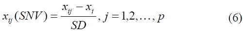
Here,

is the mean value of the uncorrected ith spectrum.
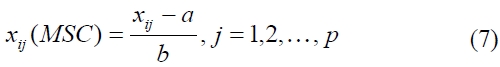
where
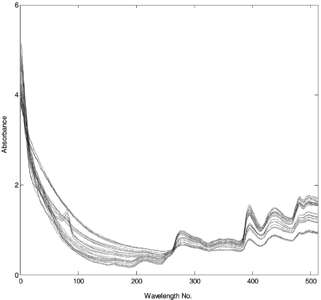
NIR measurement data for various biomasses was obtained with an advanced spectral devices (ASD) field spectrometer (wavelength range from 350 nm to 2,500 nm, Boulder, USA). In order to collect the reflectance spectra, a fiber optic probe oriented at sixty degrees to the sample surface was used. Three scans for each of samples were collected from different location of samples. In this work we considered three woody biomass
such as red oak, yellow poplar, and hickory along with three herbaceous biomass of switchgrass, corn stover, and bagasse. Three different samples were collected from each biomass. Here, wood samples were collected from different trees. A thermogravity analyzer was used to investigate the weight loss (%) profile of different biomass over temperature. Specifically, samples were first heated from 50 ℃ to 105 ℃ with the rate of 25 ℃/min and kept at 105 ℃ during ten minutes to remove the moisture. Then they were heated to 750 ℃ within a nitrogen atmosphere. Three spectra collected on each of a total of 18 samples were used to predict the weight loss profile of different biomass. The reflectance spectra were converted to absorbance spectra. The data set was further reduced by averaging the 1 nm interval spectra to one with 4 nm intervals. NIR plots of the samples are shown in Figure 1. The NIR data were used to perform a statistical analysis.
In this work, the prediction of a weight loss profile of biomass with temperatures was conducted based on multivariate statistical calibration models by analyzing the NIR spectra data. Before building a prediction model for the NIR data and weight loss profile with temperature, various preprocessing methods was applied to the original NIR data to choose optimal pretreatment scheme. Based on the 54 NIR samples three PLS models were built using the three pretreatment methods and compared. When implementing OSC, a direct orthogonal signal correction algorithm[8] was applied. The OSC-treated PLS model of 54 NIR samples was able to explain 92.1% of the Y variation. In addition, it showed a higher predictive power of 86.1% than 75.8% and 75.2 obtained from SNV and MSC, respectively. As a result, OSC was chosen in this work because the best performance was achieved from the NIR data. It is mainly because OSC-based preprocessing is able to remove unwanted variations of the NIR data that do not contribute to prediction.
The use of simple regression techniques makes it difficult to build reliable prediction models because of the high dimensionality and collinearity of NIR data. Thus, we tried to adopt an effective compression tool of a wavelet transform. A leavethree- out procedure was performed on the 54 NIR spectrain order to evaluate the performance of the proposed prediction model using test data. Specifically, three of the 54 spectra are kept out of prediction model development, and these are then predicted by the prediction model. Then, this process is repeated until every sample had been kept out only once. Such a leave-three-out test procedure is used to evaluate the prediction model by using samples that are not included in the model-building stage. It may indicate how reliable the prediction model would be practically in predicting unknown samples.
A cross-validation procedure based on the predicted residual error sum of squares was used in this work in order to select the number of latent variables for PLS models. It is due to the fact that acritical parameter that determines the performance of PLS models is the number of latent variables retained. This number should be determined by considering both the curse of dimensionality and the loss of data information. In this work as a measure of the predictive performance of a prediction model we calculated root mean squared error in prediction (RMSEP) values of residuals, which is defined as
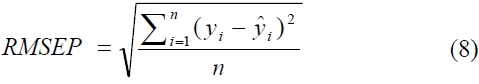
where

the predicted value, and n is the total number of samples. Methodological execution such as PLS and wavelet analysis was performed in an environment of MATLAB (The MathWorks Inc., Natick, MA) and WaveLab v. 802, respectively. This is also the case for other techniques considered here.
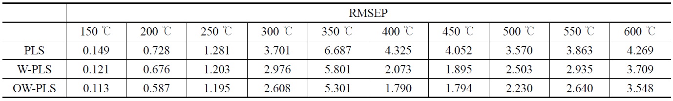
The prediction results of RMSEP values corresponding to the ten temperature points are shown in Table 1. A total of three PLS prediction models were built and compared. They are based on ordinary PLS (“PLS”), wavelet-transformed PLS (“W-PLS”), and OSC- and wavelet-treated PLS (“OW-PLS”). For the wavelettransformed models a Symmlet-8 wavelet was used in building the wavelet PLS prediction models. For different wavelet-transformed PLS models and several cross-validation runs, about 45~50 wavelet coefficientsare selected by a thresholding and used in further prediction modeling.
[Table 1.] Performance comparison of RMSEP results at different temperatures

Performance comparison of RMSEP results at different temperatures
From Table 1, we are able to find that the wavelet PLS model with OSC-treated data (i.e., OW-PLS) showed the best prediction performance: it produced lower RMSEP values at the ten temperature points. For example, OW-PLS prediction model predicted the weight loss at 150 ℃ with RMSEP = 0.113, whereas the PLS model with RMSEP value equal to 0.149. The advantage of using wavelet analysis in prediction model building can be found from this table. Compared to the PLS model, W-PLS and OW-PLS models produced lower prediction errors of RMSEP values at all the ten temperature points. At 350 ℃ RMSEP values of WPLS and OW-PLS are 5.801 and 5.311, respectively. On the other hand, 6.687 are obtained from the PLS model. The effect of using OSC pretreatment can be seen by comparing the RMSEP values of W-PLS with OW-PLS. In fact, the use of OSC showed a better predictive performance than the models without it. It should be noted that there are some differences in predictive performance of calibration models between temperatures. In case of OW-PLS, prediction error of RMSEP at 350 ℃ (i.e., 5.311) has highest one while lowest RMSEP value occurs at 150 ℃. Such a case also can be found from other prediction models. That is, the response of the weight loss at 150 ℃ showed a minimum RMSEP value and a maximum RMSEP value for the weight loss at 350 ℃. It means that the weight loss at 150 ℃ can be predicted more reliably than those at 350 ℃. Such an observation can be seen from plots of observed vs. predicted response values.
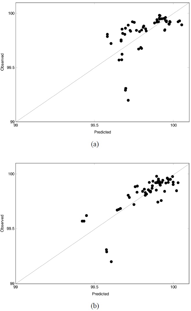
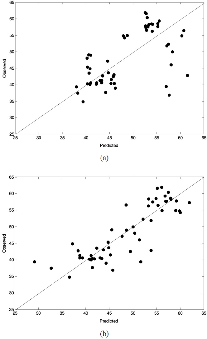
Figure 2 and Figure 3 displayed observed vs. predicted values of weight loss at 150 ℃ and 350 ℃, respectively. In both figures the plot related to PLS (OW-PLS) is shown in top (bottom) panel. Compared to the two PLS plots, OW-PLS plots at two temperature points produced reliable prediction results. It is because that in such plots the data should fall on the diagonal when calibration models predict the data perfectly. As illustrated in Figure 2, for example, the OW-PLS model has a better predictive ability at 150 ℃ than the PLS model. This is evident from comparing the three samples located at the bottom of the plots. For the three samples, the OW-PLS produced the predicted value relatively more close to the diagonal line than PLS did. Actually, the three predicted value of the PLS model is quite different from the observed one. Here, only three samples were mentioned for a comparison purpose, but it is the case for other points in
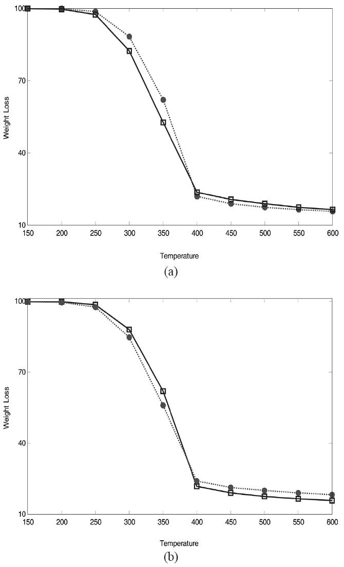
all the plots. To visualize the predictive performance of the prediction models, predicted weight loss profiles are plotted against those observed with temperatures, which is shown in Figure 4.
As expected from the comparison of RMSEP and observed vs. predicted plots, low RMSEP values resulted in little deviation between predicted and observed response variables. Overall, NIR spectroscopy combined with wavelet and statistical methods is a very useful tool to characterize biomass. It is due to the fact that NIR spectra of biomass include a lot of information in terms
of chemical composition and physical properties that affect thermal decomposition behavior. Such good performance of the wavelet PLS-based prediction model can be explained by comparing original and reconstructed data. Though not shown here, only 48 wavelet coefficients out of a full set of 538 original variables or wavelengths were used for reconstruction. Reconstruction results were quite successful in that the reconstructed values approximated the original NIR data very well. It means that the remaining information is good enough to explain important patterns of the NIR data for the prediction of weight loss profiles. In this case, 91.07% of the original information was considered as unnecessary or irrelevant parts.
In this work, the empirical models for predicting a weight
loss profile of different biomass types were developed. By using the NIR spectra data multivariate statistical prediction models were built combined with wavelet analysis and pretreatment of OSC. Prior to building prediction models for the weight loss profiles with temperature, various preprocessing methods were tested to choose optimal pretreatment scheme. The three prediction models were compared, and as a result, the wavelet PLS models with OSC pretreatment of NIR spectra showed the best prediction performance in that it produced the lowest prediction errors. This shows the possibility and benefits of using NIR spectra combined with powerful techniques to predict thermal decomposition behavior of various biomass samples. It may be due to the fact that NIR spectra are quite redundant by nature and thus suitable for compression. Another thing is that PLS is a powerful technique for modeling collinear and high-dimensional NIR data. As shown in Figure 4, there is little difference in prediction performance between PLS and OW-PLS. From a practical point of view, PLS can be one of options used for modeling NIR data because it has simple modeling procedure and comparable prediction performance. Nonetheless, more accurate prediction models should be attacked in near future using various NIR samples (more samples including six woody and herbaceous biomass types) and more advanced modeling techniques in order to improve the prediction performance for biomass.