Continuous queries [1] are standing queries, which typically run indefinitely. These queries are central to applications deal-ing with continuous and unbounded data streams [2]. Many of these applications handle data whose values may
Unlike traditional continuous queries that typically return only the values of specified attributes, a continuous
To guarantee the correctness of the result of a temporal query, adjacent or overlapping timestamps of value-equivalent tuples should be merged prior to the evaluation of the temporal function or predicate specified in the query. This merge process is referred to as
For stream applications, it is not uncommon to have insuffi-cient system resources to process or keep all tuples arriving from the input data stream in memory [2]. In these situations, discarding a fraction of tuples, called load shedding [8], often becomes necessary to resolve the problem. With load shedding in place, however, the system cannot produce an exact result, thus ensuring the accuracy of an approximate query result is an important issue [9].
In this paper, we study the problem of load shedding from a data stream in the presence of temporal coalescing, with a par-ticular focus on the case of insufficient memory to keep all tuples in the window specified in a continuous temporal selec-tion query. The presence of coalescing as an integral step in temporal query processing poses two major challenges for the load shedding mechanism.
The first challenge is that the accuracy metrics used in the existing load shedding methods (e.g., the number of tuples in the approximate result as in [10-16] or the relative deviation between estimated and actual aggregate values as in [17, 18]) are not suitable for continuous temporal queries. Since a tempo-ral query returns both attribute values and their valid time inter-vals, the accuracy metric should take both into account. The second challenge is a direct consequence of the first challenge, that is, the existing load shedding algorithms (whether random load shedding as in [17] or semantic load shedding as in [11]) are therefore inadequate for temporal queries.
To address the first challenge, we introduce a new accuracy metric that combines a value similarity metric and an interval similarity metric. The proposed metric is not only intuitive and semantically correct but also has theoretical backing. Specifi-cally, the value similarity metric is based on the Jaccard coeffi-cient [19], and the interval similarity metric is based on
In response to the second challenge, we present a new “
A performance study compares the proposed coalescence-aware algorithm to a conventional random load shedding algo-rithm. (Note that other existing load-shedding algorithms are not comparable, since they do not work with coalescing.) The main purpose of the performance study is to compare the two mechanisms in terms of the achieved accuracy. The experiment results show that the accuracy improvement of our proposed mechanism over the random mechanism approaches an order of magnitude as the coalescing probability increases and the avail-able memory size decreases. We have also examined the effects of the two greedy objectives on the performance of the pro-posed coalescence-aware algorithm and confirmed that the objectives are well balanced in their influence on the accuracy achieved by the greedy algorithm.
The main contributions of this paper can be summarized as follows.
■ It introduces the new problem of load shedding for continuous temporal queries over a windowed data stream.
■ It identifies coalescing as an important barrier to overcome, and proposes a new accuracy metric and a new algorithm for load shedding while taking coalescing effects into consider-ation.
■ It presents a thorough performance study on the proposed coa-lescence-aware algorithm and two partially coalescence-aware algorithms (each reflecting one of the two greedy objectives).
The rest of this paper is organized as follows. Section II pro-vides a relevant background and introduces the model of contin-uous temporal queries assumed in this paper. Section III presents the proposed accuracy metric and load shedding algo-rithm. Section IV presents the experiments and discusses the results. Section V reviews related work. Section VI concludes this paper and suggests future work.
II. CONTINUOUS TEMPORAL QUERIES OVER DATA STREAMS
We characterize continuous temporal queries by their support for temporal functions and predicates. These queries can be seen as a hybrid of traditional continuous queries over data streams [1] and temporal queries over temporal databases [4]. In this section, we first summarize the models of these two base query types and then introduce and motivate the model of the hybrid query type.
>
A. Continuous Queries Over Data Streams
A data stream is an unbounded sequence of tuples, and typi-cal queries on data streams run continuously for an indefinitely long time period [1, 2]. We assume that each tuple arriving from a data stream is timestamped. Additionally, we assume that all tuples arrive in an increasing order of their timestamp and that tuples in a window are maintained in an increasing order of their timestamps.
In many cases, only tuples bounded by a window on a data stream are of interest at any given time [2]. A window may be tuple-based or time -- based depending on whether its size is the number of tuples or the window time span. The solutions pre-sented in this paper --the proposed accuracy metric and the load shedding algorithm- work well with either window model.
An example continuous query is shown below, considering a wireless sensor network in which sensors are mounted on weather boards to collect timestamped topology information along with humidity, temperature, etc. [21]
Example 1. Continuous Query
SELECT S.humidity, S.timestamp
FROM Stream S RANGE 15 MINUTE SLIDES 1 MINUTE
WHERE S.humidity > 75;
>
B. Temporal Queries Over Temporal Databases
Time is a ubiquitous aspect in almost all real-world phenom-ena that many real-world applications deal with data whose val-ues may change over time. All these applications thus have intrinsic needs to model time, and it has motivated the database community to undertake an extensive study of temporal data management for relational databases [4], semi-structured data-bases (e.g., XML [23]), and data streams [24].
Temporal databases make it possible for the user to store the history of data and to retrieve this history through temporal que-ries. The importance of such capabilities has become evident with significant commercial interests ensuring that major DBMS products [25, 26] are currently supporting temporal data management as core features.
Two time dimensions are of interest in the handling of tem-poral data -- valid time interval and transaction time interval [4]. The former is the time interval during which the stored fact is true in reality. The latter is the time interval during which the fact is present in the database. A temporal database can support the former only (called a valid-time database), the latter only (called a transaction-time database), or both (called a bitempo-ral database). In this paper we consider a valid-time database.
In addition, temporal databases can support either attribute or tuple timestamping depending on whether the time interval is associated with individual attributes or with the entire tuple of all attributes [4]. In this paper we consider tuple timestamping.
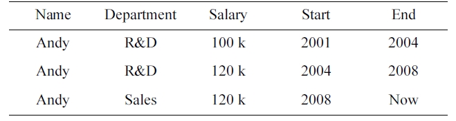
Temporal databases can be queried using Temporal SQL (TSQL) [27], which is essentially SQL that has been extended with temporal predicates and functions. The correct evaluation of temporal predicates and functions demands temporal tuples to be coalesced first. As already mentioned, coalescing is a fun-damental operation in any temporal data model, and is essential to temporal query processing since queries evaluated on uncoa-lesced data may generate incorrect answers [5, 6] (see the exam-ple below).
Example 2. Importance of Coalescing
SELECT E.NAME, VALID (E)
FROM Employee E (Name, Department) as E
WHERE CAST (VALID (E) AS INTERVAL YEAR) > 6;
[Table 1.] Andy’s employment records

Andy’s employment records
>
C. Continuous Temporal Queries Over Data Streams
As already mentioned, we see the continuous temporal stream query model as a hybrid of the continuous stream query model and the temporal database query model. What this entails in the temporal representation of tuples is that, when a new tuple,
In this paper, we consider continuous temporal
Example 3. Temporal Continuous Selection Query
SELECT S.humidity, VALID (S)
FROM Stream (humidity) as S RANGE 15 MINUTE SLIDES 1 MINUTE
WHERE CAST (VALID (S) AS INTERVAL MINUTE) >= 3;
III. COALESCENCE-AWARE LOAD SHEDDING
As mentioned in Section I, making load shedding coales-cence-aware requires a new accuracy metric and a new load-shedding algorithm because the existing ones do not work with coalescing. In this section, we propose a new accuracy metric in Section III-B and a new algorithm in Section III-C.
Property l. Bounding Property on Approximate Coalesced Tuples
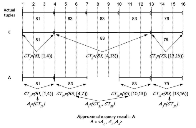
As a result of load shedding, an exact coalesced tuple
Proof: This property can be proved through a case analysis. As a result of load shedding, one and only one of the following four cases can happen to
■ Case 1: CTi is retained without any alteration. This case hap-pens when none of the tuples coalesced in CTi is dropped.
■ Case 2: An exact coalesced tuple disappears in its entirety. This case occurs when a tuple not coalesced with its adjacent tuples in the exact result is dropped.
■ Case 3: An exact coalesced tuple is decreased in its interval. This case occurs when a tuple which is either the first or the last of the tuples coalesced in the exact result is dropped.
■ Case 4: An exact coalesced tuple is split into two approximate coalesced tuples of shorter intervals. This case occurs when a tuple in the middle of the tuples coalesced in the exact result is dropped.
It is obvious in all four cases that the bounding property holds.
Since the result of a continuous temporal query consists of both the values of coalesced attributes and their associated valid time intervals (recall Definitions 3.2 and 3.3), an accuracy met-ric for this class of queries should take both into account. In this regard, we propose an accuracy metric based on the concept of the
The
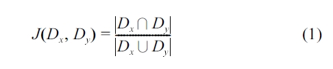
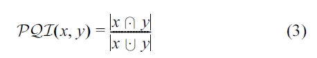
We use the Jaccard coefficients to compare the coalesced attribute
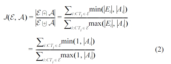
where

and ? are the multiset intersection and union opera-tors, respectively (Let
Equation 2 considers only the coalesced attribute values, and so it should be modified to consider the interval similarity factor as well. For this purpose, we adopt
(See Appendix for more information about
We use the
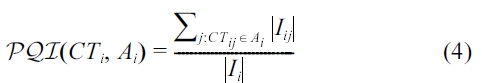
Equation 4 essentially computes the interval reduction ratio of the exact coalesced tuple
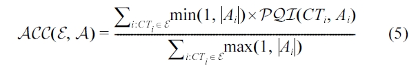
Note that min(1, |
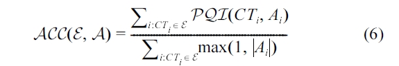
This accuracy metric has the nice property of limiting the computed accuracy to a maximum of 1.0 (i.e., 100%) and allowing for intuitive interpretations as illustrated in the follow-ing example.
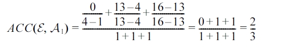
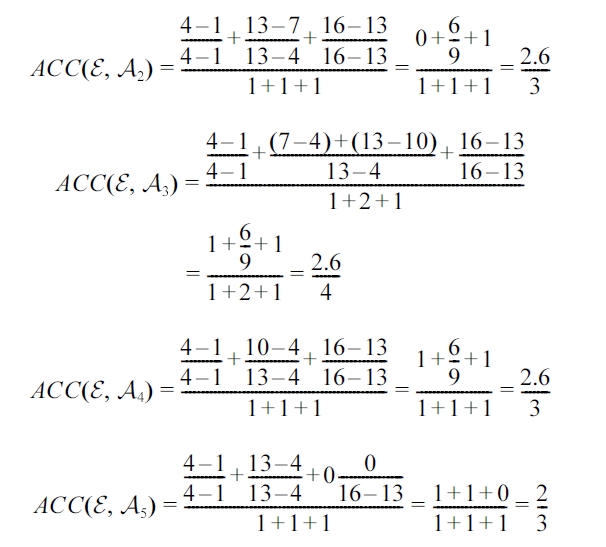
Example 4. Proposed Accuracy Metric.
>
C. Coalescence-Aware Load Shedding Algorithm
The problem of coalescence-aware load shedding can be stated formally as follows.
Problem definition: Given the memory M (of size |M| tuples) and a continuous temporal query which specifies coalescing tuples in a window WS (of size |WS| tuples) over a data stream S, we discard |WS| ? |M| tuples from the |WS| tuples with the objective of maximizing the accuracy of the query output subject to the constraint that |M| < |WS|.
Finding an optimal solution would require holding all |

possible sub-sets an optimal subset of tuples to discard. This problem is harder than the NP-hard nonlinear binary integer programming problem, as there is no well-formed functional form for com-puting the accuracy for a given set of binary integer assign-ments (e.g., 1 for retaining a tuple and 0 for discarding a tuple). So, we propose a greedy algorithm, which takes a quadratic run-ning time in the worst case and consumes a linear amount of storage space.
The proposed algorithm decides which tuple to drop from memory upon the arrival of each new tuple from the input data stream. The algorithm uses a greedy strategy based on two objectives for achieving value similarity (Equation 2) and inter-val similarity (Equation 4).
There are different ways to combine
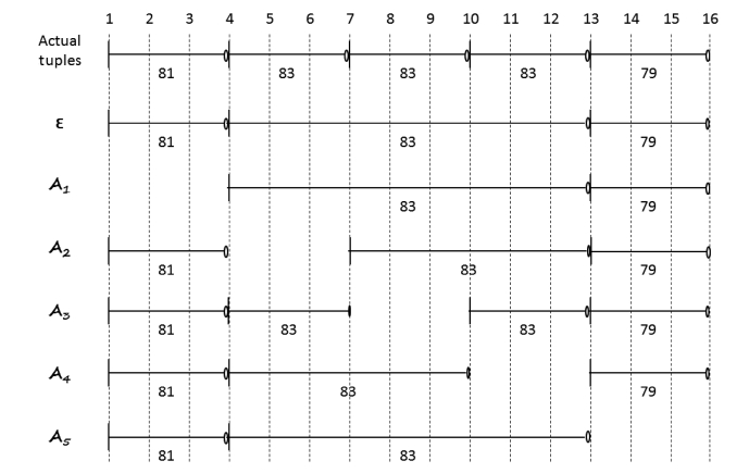
For example, Table 2 shows the values of
[Table 2.] δ+sj and ρ?sj for tuples in Example 4.
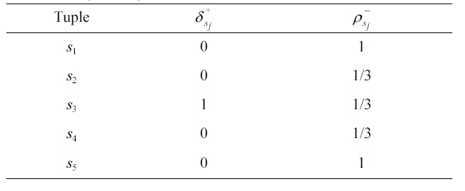
δ+sj and ρ?sj for tuples in Example 4.
of the five actual tuples in Example 4. It shows that the tuples that have a minimum value of
Algorithm 1 outlines the steps of load shedding using the combined objective function. Upon the arrival of a new tuple
[Algorithm 1.] Coalescing-aware load shedding (CALS)
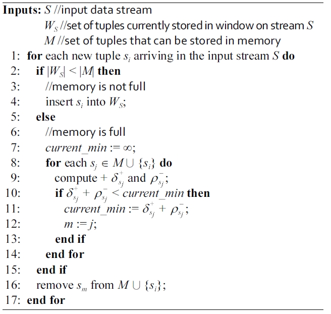
Coalescing-aware load shedding (CALS)
It is easy to see that the running-time complexity is
In the experiments presented in Section IV, we use two addi-tional algorithms, called coalescence-aware load shedding (CALS)-V and CALS-I. CALS-V is the CALS algorithm reduced to consider only the value similarity (hence using
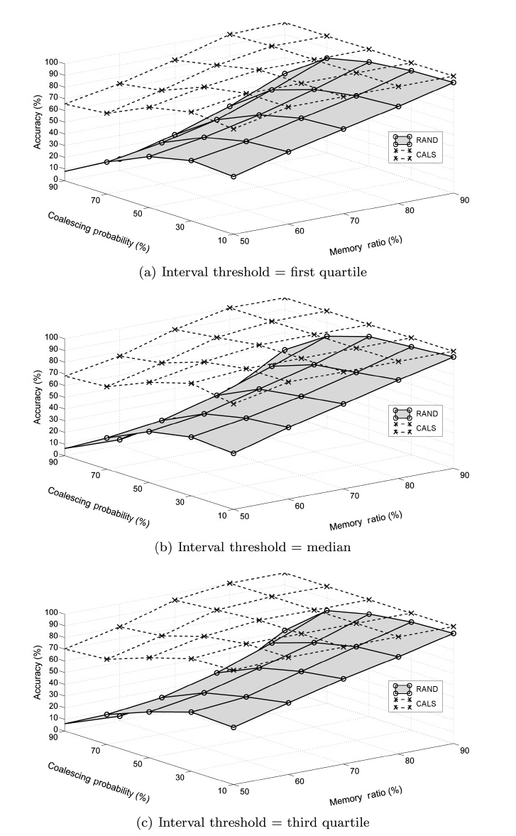
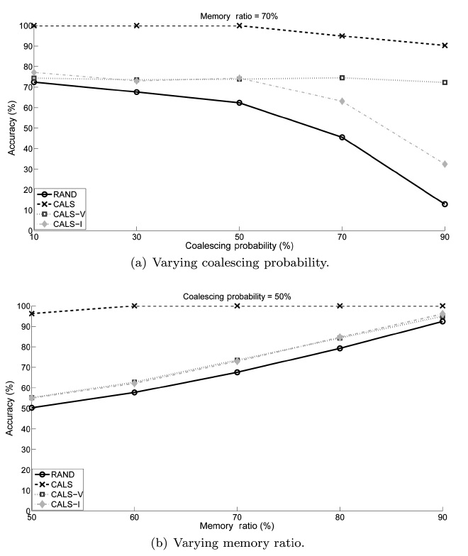
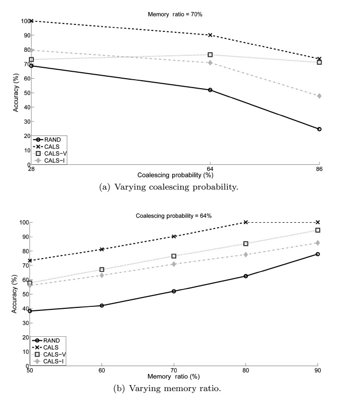
We conducted experiments to study the performance of the proposed load shedding algorithm. The main objective of the experiments was to observe the effectiveness of the proposed CALS algorithm. Additionally, we compare CALS with two partially coalescence-aware algorithms, CALS-V and CALS-I, to observe how each of the two complementary greedy objec-tives affects the performance individually. We use the random load shedding (RAND) algorithm as the baseline approach (Under this random load shedding mechanism, tuples are dis-carded randomly such that each tuple has the same probability of being discarded from (or, equivalently, retained in) mem-ory.). As anticipated, the experiment results show that CALS achieved the highest accuracy, RAND achieved the lowest, and CALS-V and CALS-I are in between.
The experiments were conducted using Matlab (Release R2010b) on a 64-bit machine with 4.00 GB internal main mem-ory. We use the Matlab array/matrix data type to implement the window data structure.
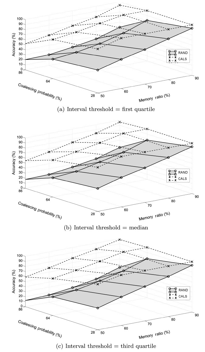
For each algorithm, we measured the achieved accuracy as an average of the accuracies measured using each data set. The results are presented in two stages in this section. The first stage focuses on comparing CALS with RAND to see the effect of coalescence-awareness on the accuracy. The second stage focuses on examining the individual effects of the two partially coalescence-aware greedy objectives.
value. This indicates that, while the load shedding produces more tuples of shorter coalesced intervals, the relative differ-ence between the sets of tuples selected in the case of exact and approximate query results does not change much for different threshold values.
In addition, we see that their performance is very close to each other regardless of the memory ratio. This is evident from the fact that the memory size determines the number of tuples to be dropped, and it has equitable effects on the proposed accu-
racy under both greedy objectives.
We also see that the performance of CALS-V changes little as the coalescing probability increases while CALS-I starts degrading as it increases beyond around 50%. Our reasoning is that CALS-V aims at deciding which tuples to retain that would otherwise cause time gaps (hence extraneous tuples) and so has little dependency on the coalescing probability itself, while in CALS-I it is more likely that tuples influencing the accuracy more (even if they have the shortest time interval) are dropped as the coalescing probability increases.
There are two separate aspects to the related works we look at: load shedding from a data stream and temporal coalescing over data streams.
>
A. Load Shedding from a Data Stream
The most common accuracy metric assumed in the research literature for load shedding over data streams is the size of approximate query result [10-16]. A few other existing studies, specific to aggregation queries, assume the accuracy metric of the relative error between approximate and actual aggregate values [17, 18]. For both of these accuracy metrics, the accom-panying algorithms are generally categorized as random load shedding (i.e., drop tuples randomly, as in [17, 29]) or semantic load shedding (i.e., drop tuples based on their relative impor-tance, as in [11]).
For maximizing the size of an approximate result (known as the max-subset), Das et al. [11] proposed two heuristics for dropping tuples from window-join input streams. The first heu-ristic sets the priority of a tuple being retained in memory based on the probability that a counterpart joining tuple arrives from the other data stream. The second heuristic favors a tuple based on its own remaining lifetime. Kang et al. [14] proposed a cost-based load shedding mechanism for evaluating window stream joins by adjusting the size of the sliding windows to maximize the number of produced tuples. Ayad and Naughton [10] pro-posed techniques for optimizing the execution of conjunctive continuous queries under limited computational resources by placing random drop boxes throughout the query plan to maxi-mize the plan throughput. Xie et al. [16] presented a stochastic load shedding mechanism for maximizing the number of result tuples in stream joins by exploiting the statistical properties of the input streams. Gedik et al. [12] proposed a load shedding approach for stream joins that adapts to stream rate and time correlation changes in order to increase the number of output tuples produced by a join query. Then, Gedik et al. [13] further addressed the problem of multiple-way joins over windowed data streams and proposed a window segmentation approach for maximizing the query output rate. Tatbul and Zdonik [15] pro-posed a load shedding operator that models a data stream as a sequence of logical windows and either drops or retains the entire window depending on the definition and characteristics of the window operator. For minimizing the relative error for aggregation queries, Babcock et al. [17] proposed a random sampling techniques for optimum placement of load shedding operators in aggregation query plans, measuring the resulting accuracy as the relative deviation between estimated and actual aggregate values. Law and Zaniolo [18] proposed a Bayesian load shedding approach for aggregation stream queries with the objective of obtaining an accurate estimate of the aggregation answer with minimal time and space overheads.
In contrast to all this existing work, we address a rather novel query model for data streams under which a query result is com-posed of both attribute values and the valid time interval of each value. Therefore, all the existing load shedding accuracy met-rics and algorithms are not applicable to our research problem.
>
B. Temporal Coalescing Over Data Streams
Barga et al. [30] proposed to employ temporal coalescing in view of complex event processing over data streams, so that two events are represented as a single event if their valid-time intervals overlap. Zaniolo [31] examined how temporal coalesc-ing can be expressed for a sequence of events using OLAP functions and Kleene-closure constructs. Kramer and Seeger [32] introduced coalescing as a physical operator for compact-ing the representation of a data stream by merging tuples with identical values and consecutive timestamps into a single tuple. Recently, we studied coalescing for a
While all this existing work is pertinent to temporal coalesc-ing over data streams, none of them addresses it from the view-point of memory being insufficient to retain all tuples. To the best of our knowledge, our work is unique in this regard.
This paper addressed the problem of load shedding from a window for continuous temporal queries over data streams when memory is limited. The key challenges come from the fact that tuples need to be coalesced for temporal query process-ing and that this fact makes existing load-shedding algorithms and the accuracy metric used by them inapplicable. Thus, we proposed a new accuracy metric and a new algorithm that can handle coalescing challenges well. The accuracy metric com-bines a value similarity metric based on Jaccard coefficients and an interval similarity metric based on
For future work, there are several extensions possible. First, this paper focuses on the limited-memory case, and so the lim-ited-CPU time case is another problem we could look into. Sec-ond, this paper considers the temporal selection query, and other query types like aggregation or join queries are possibilities for further work. For this, the accuracy metric and the greedy strat-egy may need to be adapted to the query type. Third, this paper considers queries retrieving both the attribute values and their valid time intervals. Considering special cases, such as a snap-shot query (retrieving only attribute values) and the valid-time query (retrieving only valid time intervals) [27], may offer sim-pler and more efficient solutions. This too could be an interest-ing study.
>
Appendix. PQI Interval Orders
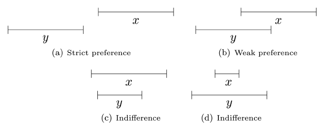
The
The strict preference relation (denoted as
The degree of overlap between two intervals can be used as a measure of the
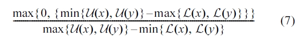
This equation is equivalent to Equation 3 in Section III-B.