We propose two new approaches that automatically parallelize Java programs at runtime. These approaches, which rely on run-time trace information collected during program execution, dynamically recompile Java byte code that can be executed in parallel. One approach utilizes trace information to improve traditional loop parallelization, and the other parallelizes traces instead of loop iterations. We also describe a cost/benefit model that makes intelligent parallelization decisions, as well as a parallel execution environment to execute parallelized programs. These techniques are based on Jikes RVM. Our approach is evaluated by parallelizing sequential Java programs, and its performance is compared to that of the manually parallelized code. According to the experimental results, our approach has low overheads and achieves competitive speedups compared to the manually parallelizing code. Moreover, trace parallelization can exploit parallelism beyond loop iterations.
Multicore processors have already become mainstream in both personal and server computers. Even on embedded devices, CPUs with 2 or more processors are increasingly used. However, software development has not come up to par with hardware. Designing programs for multi-processor computers is still a difficult task, one that requires much experience and skill. In addition, a large number of legacy programs that are designed for singleprocessor computers are still running and need to be parallelized for better performance. For these reasons, a good approach for program parallelization is needed. A compiler that automatically parallelizes a source code into an executable code for multi-processor computers is a very promising solution to this challenge. A lot of research in this field has shown the potential of compilerbased parallelization. However, most of the successes have been limited to scientific and numeric applications with static compilation. Recently, virtual machines have been parallelized [4-6, 15]. VMs provide rich run-time information and a handy dynamic compilation feature, which, together with traditional compiler techniques, shows good potential of automatic parallelization. In this paper, we propose two automatic parallelization approaches based on the Java virtual machine (JVM).
Traces, which are sequences of actually executed instructions, are used in our approaches to improve loop parallelization or are used even as units of parallel execution. Furthermore, we collect trace information during pro-gram execution, so our approach works simply with any given Java byte code. No source code or profiling information is needed. Some excellent existing features in JVM, such as run-time sampling, on-demand recompilation and multi-thread execution, are used. Enhanced by run-time trace information, our experimental results show that this approach can provide a more competitive parallelization of Java programs than manual code parallelization can. The remainder of this paper is organized as follows. An overview of our approaches is described in Section II. Section III presents the technical details of the on-line trace collection system. Section IV describes the analysis of the dependencies between traces. Section V describes Trace-Enhanced Loop Parallelization (TELP), including a cost/benefit model, a parallelizing compiler and a parallel execution environment. Section VI explains another parallelization approach that parallelizes traces instead of loop iterations. Section VII describes the evaluation methodology. Section VIII demonstrates and analyzes the experiment results. Section IX discusses related works. And finally, the last section concludes this paper.
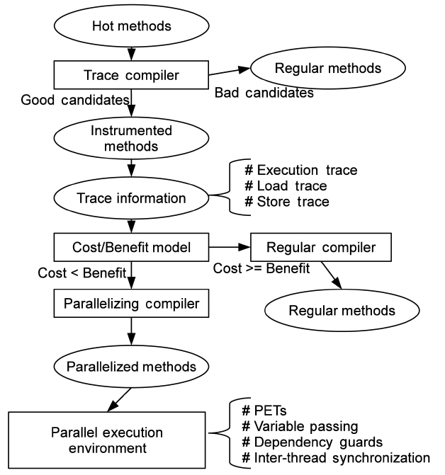
Fig. 1 depicts the TELP system that is implemented on Jikes research virtual machine (RVM) [5], and also the main procedure of parallelization. There are four main components in our system: an on-line trace collector, a cost/benefit model, a parallelizing compiler and a parallel execution environment. First, we use the on-line sampling- based profiling mechanism of Jikes RVM to identify “hot methods”, which takes much of the total execution time of Java programs. We only consider hot methods as candidates for parallelization to reduce unnecessary instrumentation and threading overheads.
In the TELP approach, we filter the hot methods based on several heuristics. First, only methods from user applications are selected. Thus, the Java core and VM methods are not considered in this work. Second, the length of the methods cannot be very short. Third, the methods must contain loops. The hot methods satisfying these criteria are good candidates for parallelization. After good candidates are identified, we recompile them to insert an instrumentation code.
As a result, trace information can be collected in the subsequent executions of the instrumented methods for delivery to a cost/benefit model, which decides whether or not the traces are profitable for parallelization. After that, those traces found to be worthy of parallelization are passed to a parallelizing compiler, which recompiles the methods that contain these traces. And finally, parallelized traces execute in parallel inside the Parallel Execution Environment (PEE). The details of these components of TELP are described in the following sections of this paper.
Trace Parallelization (TP) works in the same way as
TELP until trace information is collected. When trace information has been collected, it builds a trace dependence graph for each parallelizing candidate. Instead of compiling the whole method, TP compiles traces and generates a machine code for each trace individually. The traces, then, are executed in parallel according to their dependence graphs, and dispatched to multiple cores dynamically at run-time. At the same time, the original sequential code is kept as a fail-safe solution. The VM automatically falls back to its original code when an abnormal exit from a trace is detected.
III. ON-LINE TRACE COLLECTION SYSTEM
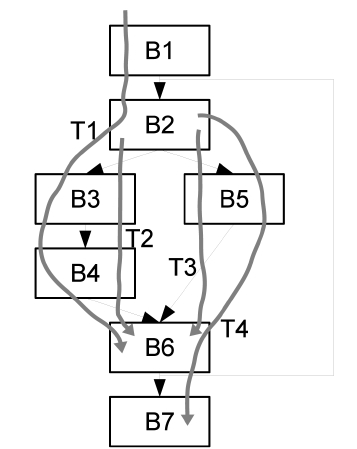
A trace is defined as a sequence of unique basic blocks which are executed sequentially during the execution of a program [6]. An example of trace formation is shown in Fig. 2, which is a control flow graph of a section of a program. Trace T1 is the sequence of {
Execution Trace
An execution trace records a sequence of executed instructions and basic blocks. Instrumenting code sections are injected at every jump and branch instruction, recording their run-time targets. Similar instrumentation is applied to method calls and returns. Particularly, backward jumps or branches are used to identify loops and collect loop information, like induction variables and loop boundaries. Time stamps are also collected at instrumenting points for future analysis during parallelization.
Memory Access Trace
A memory access trace is a sequence of read and write operations to the memory, including variables, fields and array references. It is collected for data dependence analysis during parallelization. Because actual memory addresses can be collected by on-line TCS, dependence analysis, more accurate than static approaches, can be carried out especially for class fields and array accesses. To reduce memory space overheads, continuous memory addresses are combined into one entry, and only a limited number of entries are kept in one trace. Our study shows this approach works well with regular loop-carried dependencies.
These two types of traces are bound such that each execution trace has only one memory trace. And the boundaries of traces are determined by specific types of instructions at run-time. A trace starts upon detecting one of two possible trace entry points: 1) First instruction of an instrumented method, and 2) exit points of other traces.
On the other hand, traces end at several other program points: 1) backward jumps/branches, 2) last instruction (usually return instruction) of an instrumented method, and 3) points where the length of a trace exceeds a given threshold, i.e., 128 byte code instructions in this study, which is rarely reached based on our experiments.
Based on the conditions described above, traces are constructed and stored as objects in the JVM. Also, additional information, such as execution count of traces, is also recorded and saved within the trace objects. As a result, the hot methods, which are potential targets for parallelization, can be split into multiple traces. For example, a single level loop without any branch can be normally divided into three traces: one trace is the first iteration consisting of some instructions before the loop; another trace is the loop body that may be executed many times; and the last one is the last iteration that jumps out of the loop and continues executing following instructions.
A TCS can be implemented in several ways, such as by uses of a hardware profiler and a machine code recorder in an interpreting VM. However, our choices are narrowed down by the unique constraints that our on-line TCS needs to satisfy.
Low overheads
Because our TCS is on-line, any overhead introduced here can affect the final performance of the whole system. Hence, the time spent on the TCS must be minimized. In addition, trace information collected by the on-line TCS, as well as the execution program, is stored inside of JVM’s run-time heap. As a result, we also need to control the space overheads of TCS to avoid unnecessary garbage collection (GC), which may degrade the performance and complicate the dependence analysis.
Detail and accuracy
On the other hand, on-line TCS is expected to provide detailed, accurate trace information on parallelizing candidates. The parallelizing system relies on this information for subsequent tasks, including decision making, dependence analysis and final parallelization compilation. At least, all branch/call targets must be recorded, as well as the memory accesses to variables and arrays.
Due to the two requirements and the fact that Jikes RVM is compilation-based, we enhance Jikes RVM's baseline compiler by giving it the ability to insert instrumenting code into a generated machine code. Instrumenting code is executed when certain points during program execution are reached. At that time, useful run-time information like register values and memory addresses is sent to the trace collector running in VM. In order to minimize overhead while recording detailed, accurate data, the TCS is made to work selectively at different levels of detail in various parts of a program. Specifically, trace collection has three levels.
Level 0 - The lowest trace collection level where only records of method calls and returns are kept. This level is applied to most methods that are not hot.
Level 1 - In this level, full execution traces are recorded, while no memory access trace is kept. This level is used for the non-loop sections in hot methods.
Level 2 - The highest level that records both execution and memory access traces. The most detailed and accurate information is provided by this level for future analysis and parallelization. Only loops in hot methods, which are best parallelizing candidates, can trigger level 2 trace collection.
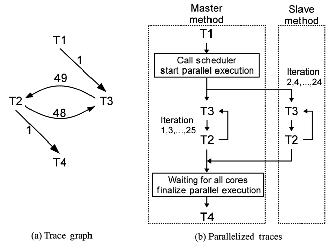
Hence, only a small but frequently executed part of a program is fully instrumented. Overheads are significantly reduced while most useful traces retain detailed, accurate information. Besides, after being recompiled and instrumented, the methods execute only once to collect trace information. Once a method finishes a profiled execution, trace information is passed to the cost/ benefit model for making parallelization decisions. Then, the method is either parallelized or recompiled into plain machine code without any instrumenting code. Regardless of the decision made, there is no more trace collection overhead after recompilation. Because of all the efforts described above, the overhead of our on-line TCS is acceptable. On the other hand, most executions of a method behave similarly, even though they have different parameters. Furthermore, traces are collected after the warm-up stage of the Java programs, so the execution is rather stable. Thus, the trace information is accurate enough for parallelization. The output of trace collection is a data structure named Trace Graph. In a Trace Graph, the nodes are the traces and the edges describe the control flow dependence among traces. For example, if a trace T2 starts right after another trace T1 exits, a directional edge will be created from T1 to T2. Each edge has a weight that records how many times the edge has passed. A full example is shown in Fig. 3a.
Given different memory access patterns, traces may be data-dependent on each other. In order to resolve the dependence among traces, we utilize the memory access trace information collected by our on-line TCS. Two types of dependencies are local variables and arrays. They are processed separately based on memory access traces. For the local variables in a trace, we generate both read and write lists from the corresponding memory access trace. Since local variables are stored in JVM runtime stack and represented by unique integer values in Java byte codes, read/write lists are sequences of integers. We first simplify the lists of a trace according to intrace dependence, and then calculate inter-trace dependencies.
Arrays have to be carefully managed because they are in the heap, and the only way to access an array element is through its memory address. Our memory access trace records the actual memory addresses accessed by the traces during the instrumenting execution. When an instrumented method is executed, its load and store instructions, as well as their memory addresses, are monitored and stored in its memory access traces. Then, we perform an analysis similar to what is done for the local variables. The only concern is the memory usage for storing these addresses. To deal with this problem, we compact one section of continuous addresses into one data record, which stores a range of memory addresses instead of a single address. This compaction can save a lot of memory spaces, as observed in our experiments.
We also try to simplify the dependence analysis by introducing a dependent section, which is a section in a trace containing all instructions dependent to another trace. For instance, a single loop has 100 instructions and the 80th and 90th instructions carry the dependence between loop iterations. In this case, the dependent section of the loop body trace is 80 to 90 after dependence analysis. A dependent section is used based on the observation that in most cases only a small section of instructions in a trace carries dependencies. In addition, using a single dependent section for each trace greatly reduces the synchronization/lock overheads in the busy-waiting mode, which is used in our parallel execution model.
V. TRACE-ENHANCED LOOP PARALLELIZATION (TELP)
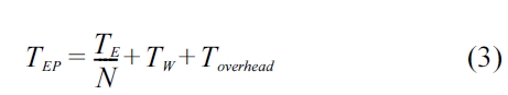
After collecting trace information for hot methods and analyzing dependencies between traces, our approach then decides whether or not they are worthy of parallelization. We introduce a cost/benefit model inspired from the one used in Jikes RVM’s adaptive optimization system [7]. This model calculates the estimated times of both sequential and parallel executions of a parallelizing candidate with its trace information and some constants. Parallelization is performed if the following inequality is satisfied.
TEP < TE × f (1)
Here,
TE = TP = S × Q (2)
In Equation 2,
In Equation 4,
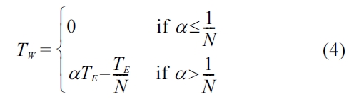
And
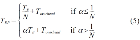
After
Parallelizing candidates that pass the check in the cost/ benefit model described above are sent to the parallelizing compiler. One candidate is then compiled to
[Table 4.] Algorithm 1: Trace-enhanced loop parallelization
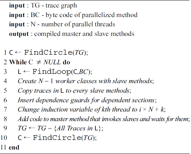
Algorithm 1: Trace-enhanced loop parallelization
execution are ignored.
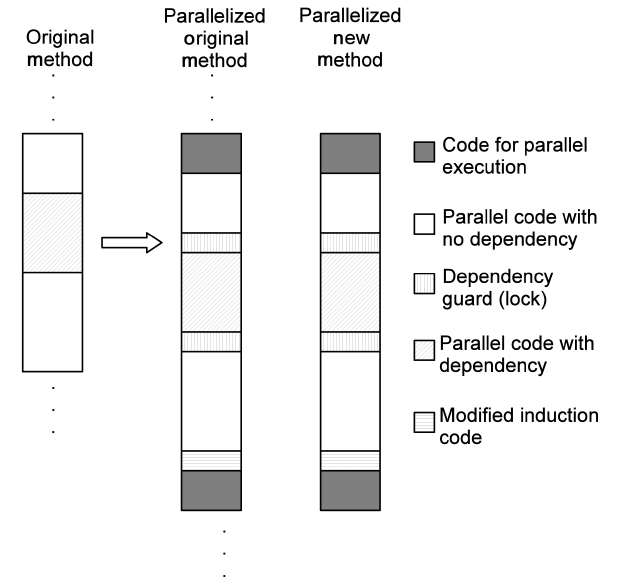
Moreover, Fig. 4 depicts the details of the code generated by a parallelizing compiler. Several special code segments are inserted into both the original method and the parallelized new methods. They are as follows:
Code preparing parallel execution: pass variables and invoke parallel execution.
Code for dependency guards: obtain and release locks.
Code of modified induction/reduction: used for parallelized loop iterations.
Code finalizing parallel execution: pass variables back and clear the scene.
As described in Algorithm 2, our approach is a hybrid of trace parallelization and loop parallelization. Pure trace based parallelization is not used because of the limitation of on-line trace collection. Due to branches, a program may have different traces for different given inputs, and online trace collection does not guarantee coverage of all possible traces at run-time. As a result, if pure trace-based parallelization is applied, the parallelized code may be missing some execution paths. In order to resolve this problem, we combine trace parallelization and loop parallelization. Loop bodies that contain traces are detected and parallelized instead of traces. Hence, all possible paths are covered, and control flows among traces are controlled by the branches in the loop bodies, simplifying the code generation for multiple traces. Also, the hybrid approach uses more run-time trace information than the traditional static loop-based approaches to perform more aggressive and accurate parallelization. A major advantage of our hybrid approach is that the data dependence analysis, which is based on run-time trace information as described in Section IV, is much more accurate than that carried out in static loop-based parallelization. For instance, if basic block B3 in Fig. 2 wants to access some data stored in the heap, it would hard and
sometimes impossible for a static loop-based parallelization approach to determine whether or not this memory access would be safe for parallelization. But this determination becomes much easier in our hybrid approach because the actual memory addresses are recorded during trace collection, and thus the memory access pattern of B3 can be constructed and used for parallelization. However, the hybrid approach introduces branches into the parallelized code, which may reduce pipeline and cache performance below that of the purely trace-based parallelized code, which is completely sequential. In addition, the number of dependent sections may increase because more instructions are compiled into the parallelized code. And memory spaces may be wasted for those instructions that will actually never be executed.
>
C. Parallel Execution Environment
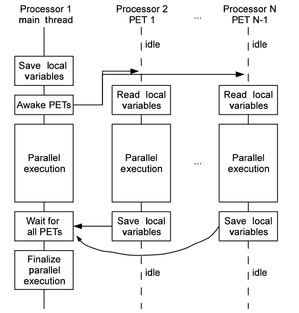
PEE is implemented upon Jikes RVM’s multi-thread execution functionality. PEE contains one or more parallel execution threads (PETs), manages copies of the local variables passed between the main thread and PETs, and maintains the dependence guards wrapped to the dependent sections in the code. Generally, PEE manages the executable codes generated by the parallelizing compiler, and ensures their correct executions. Fig. 5 demonstrates how PEE works with a parallelized code section running on
1) Parallel Execution Threads
As shown in Fig. 5, PETs are separately assigned to multiple processors. Normally, one PET does not travel between processors to reduce overhead. PETs and daemon threads t start running right after VM is booted. However, PETs stay in the idle state before any parallel
execution method is dispatched. PETs may be woken up by the main thread, and only by the main thread. After executing the given parallel execution method, a PET goes back to idle and waits for next invocation from the main thread.
There are several benefits of using the wake-up/sleep mechanism instead of creating new threads for every parallel execution, though the later approach is easier for implementation. First, using a fixed number of threads greatly reduces the memory load during run-time. Second, the scheduler can be further extended for other advanced scheduling policies.
2) Variable Passing
Local variables, which are shared across PETs, need to be copied and passed safely to other threads, besides the main thread, by using arrays. Each parallelized code section has its own variable passing array, which is pre-allo
[Table 1.] Description of Java Grande benchmarks

Description of Java Grande benchmarks
cated in the compilation stage. The array is filled with local variable values before PETs are woken. At the beginning stage of each parallel executed method, those values are read correctly from the array. Similarly, writing back to this array is the last job of a parallel executed method. And the main thread restores local variables from the arrays before moving on to the next instruction. This procedure is shown in Fig. 5.
3) Dependence Guards
Dependence guards are implemented with a Java thread synchronization mechanism, particularly, locks. During parallelizing compilation, dependent code sections are identified based on trace information, and each segment is wrapped with two special code segments called dependence guards. First code segment is inserted before a dependent section to acquire a lock, and the other one right after the dependent section to release the lock. To reduce complexity and synchronization overhead, each parallelized section holds only one lock object. This means all dependent instructions have to share one lock, and consequently the dependent section becomes a union of all individual dependent instructions. Although this approach increases the
To apply parallelism beyond loop iterations, we develop another approach that compiles individual traces into a machine code and executes them in parallel dynamically. This approach uses trace dependence graphs to find next executable traces and dispatch them to worker threads that run on multiple cores.
Loop iterations are treated as duplicated traces with different induction variable values, and thus Loop iterations can be parallelized as well. Moreover, traces that are not in loops now can also be parallelized, once their dependences are satisfied.
>
A. Parallel Execution of Traces
Algorithm 2 describes how a worker thread obtains the executable traces and then lets them run on multiple cores. In this algorithm, the ReadyList is a list of traces whose dependences are already satisfied during the previous execution. Its
[Algorithm 1.] Algorithm 2: Parallel execution of traces on each worker thread
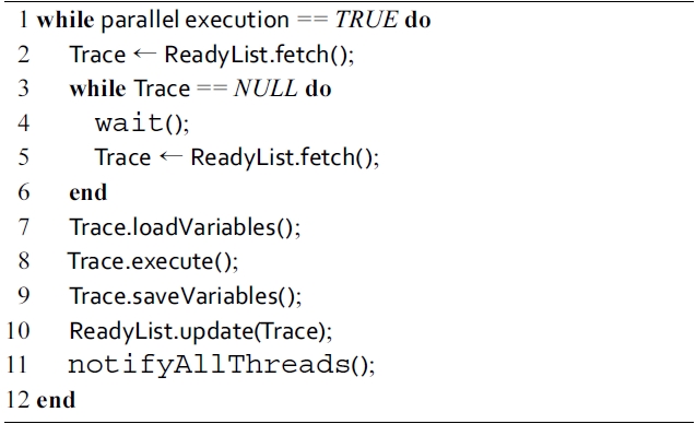
Algorithm 2: Parallel execution of traces on each worker thread
However, parallelizing a method based on the on-line trace information is not always safe because the traces collected at run-time cannot guarantee coverage of all possible execution paths in a Java program. To maintain
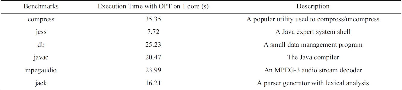
[Table 2.] Description of SpecJVM98 benchmarks

Description of SpecJVM98 benchmarks
correct parallel execution, all exit points of the traces have to be monitored. An exit point is defined as an instruction that makes the execution stream jump out of a trace. For example, a conditional branch instruction is a potential exit point, because it may change the program counter (PC) to some instruction that is out of any trace. We insert a monitoring code before every exit points in executable traces. As a result, whenever an execution stream is going out of collected traces, a fallback event is reported to the controller thread. Consequently, the parallel execution is stopped, and the original sequential code is invoked to complete the execution correctly. In order to fully recover the execution, stack states before the parallel execution are saved in memory and restored before invoking the original fall-back methods.
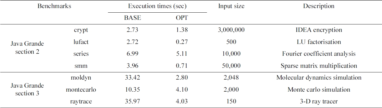
Our approaches, TELP and TP, are implemented as described in previous sections by extending Jikes RVM version 3.1.0. Also, for comparison, a simple loop parallelizing compiler is implemented. The code is compiled with Sun JDK version 1.5.0\_19 and GCC version 4.3.3. We use a dual-core Dell Precision 670 with a 2- core Intel Xeon 3.6 GHz processor and 2 GB DDR RAM to run the experiments. The operating system on that machine is Ubuntu Linux with kernel version 2.6.28. Each processor has an 8 KB L1 data cache and a 1024 KB L2 cache. The scalability of our approaches is tested by using an 8-core Intel Xeon 2.26 GHz (E5520) processor, which has four 32 KB L1 instruction caches and four 32 KB L1 data caches, as well as four 256 KB L2 caches and an 8 MB L3 cache and 6 GB memory. The operating system is 64- bit Debian Linux with kernel version 2.6.26. The benchmarks used in our experiments are from Java Grande benchmark suite [8, 9] and SpecJVM98 [10].
We divide the benchmarks from Java Grande into two groups. The first group consists of four benchmarks from
On the 2-core machine, we first measure the fraction of trace execution time to justify whether or not traces are worth parallelizing. Then we evaluate our TELP approach by two metrics: speedup and overhead. Speedup is defined as the ratio of sequential (base) execution time to parallel execution time. We measure the speedups of our automatic parallelized version and manual parallelized version, which is provided by the Java Grande benchmark suite. Overhead is defined as the time spent on trace collection and recompilation. Afterwards, we compare four parallelizing approaches, which are manual parallelization (MP), loop parallelization (LP), TELP and TP, on an 8-core machine using 7 benchmarks from Java Grande benchmark suite. We also compare the latter three approaches with 6 benchmarks from the SpecJVM98 benchmark suite, which does not have the manually parallelized code.
>
A. Results on 2-core Machine
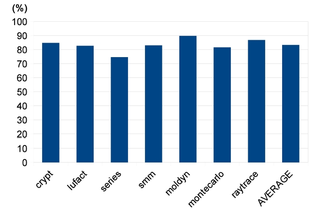
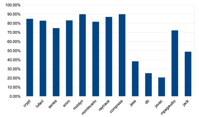
1) Trace Execution Fraction
We first measure the execution time of traces by instrumenting baseline compiled benchmark programs. We only keep hot traces, which execute more than 100 times, in the results, because frequently executed traces are potential targets for parallelization. The results are shown in Fig. 6. The execution time spent on frequently executed traces ranges from 74.60% to 89.71%, indicating that these hot traces comprise the major portion of a program execution. Hence, a decent speedup can be expected if the hot traces are well parallelized.
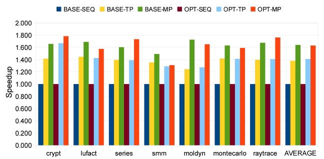
2) Speedup
The speedups of all 7 benchmarks are shown in Fig. 7,
where SEQ represents sequential execution, TP stands for trace parallelization, and MP represents manual parallelization. We also measure the speedups with and without optimization of Jikes RVM, which are represented as BASE and OPT, respectively. With our approach, all seven benchmarks achieve obvious speedups with and without optimization. The average speedups are 1.38 (baseline) and 1.41 (optimized) on two processors, as shown in Fig. 7. On a dual-core machine without optimization, the first group of four benchmarks shows fair speedups of around 1.4. Among the other three benchmarks from
In the beginning of out experiments, we do not allow any optimizing recompilation during program execution because we want to study our approach without any possible interference. However, Jikes RVM provides a powerful adaptive optimization system (AOS) that boosts the performance of Java programs. Hence, we also study the impacts of optimizations on speedup. The results in Fig. 7 indicate that our approach for automatic parallelization still works well with Jikes RVM’s AOS. The average speed up is 1.41, which is similar to the result in Section VII-A and competitive to the 1.63 average speedup of manual parallelization. Jikes RVM’s AOS and our approach integrate naturally because good parallelizing candidates are usually also good targets for optimization, and our framework can exploit the optimization compiler during parallelization.
Compared to the manually parallelized version of all seven benchmarks, our approach shows less speedup. The reason is that manual parallelization applies more aggressive parallelizing techniques, whereas our approach uses simple ones. For example, a reduction instruction like
3) Overhead
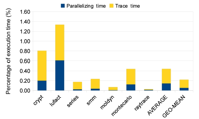
The overheads introduced in our approach are shown in Table 3 and Fig. 8. They are surprisingly small for a system with on-line instrumenting and dynamic recompilation. As described in Section II, we have made a lot of efforts on trace collection to reduce overheads. By limiting the high-level trace instrument to hot methods and executing instrumented code only once, the time overhead of trace collection is satisfied, only 0.30% on average. Moreover, compilation overhead is also smalls because
[Table 3.] Overheads of parallelization
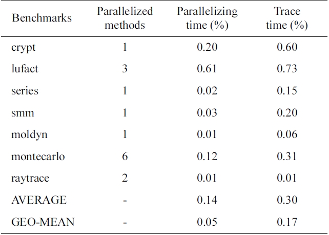
Overheads of parallelization
of the baseline compiler that is used for both instrumenting and parallelizing. Although generating non-optimized machine code, the baseline compiler is the fastest compiler provided by Jikes RVM. The average compilation overhead is 0.14%; however, a higher compilation overhead can be expected if an optimized complier can replace the current baseline compiler. It is also shown in Table 3 that overhead is related to the number of parallelized methods. We divide all 7 benchmarks into two groups based on their total execution times, where group 1 benchmarks have higher overheads because of their shorter running times. In the group of first four benchmarks, lufact has 3 methods parallelized while others have only one, and thus, both parallelizing and trace overheads of this group are the highest. In the second group, Montecarlo parallelized 6 methods, and consequently, this group’s overhead (0.43%) is much higher than those of moldyn (1 method, 0.07%) and raytrace (2 methods, 0.02%). Additionally, the accessed memory size affects trace collection overhead, and for this reason, the overhead of moldyn’s trace collection is greater than that of raytrace.
B. Results on 8-core Machine
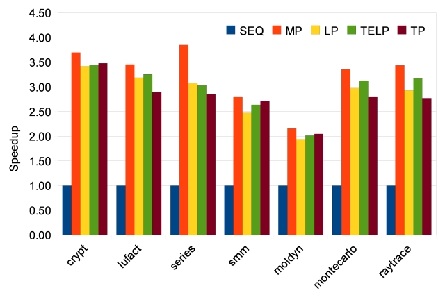
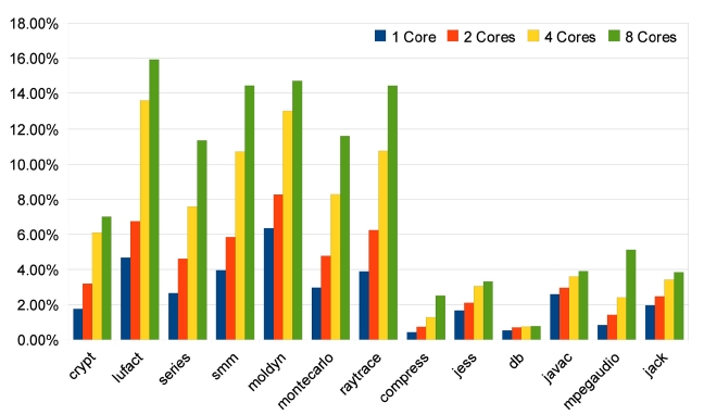
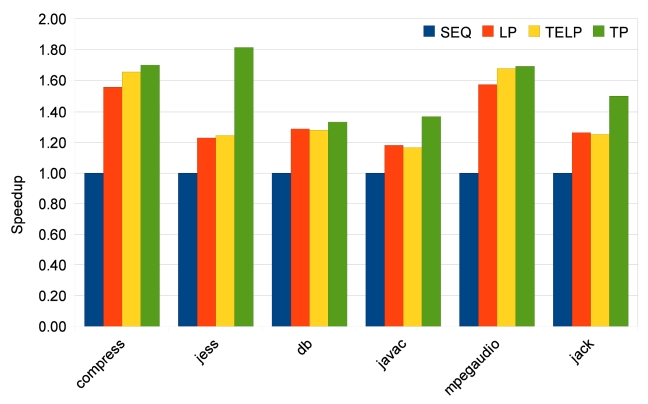
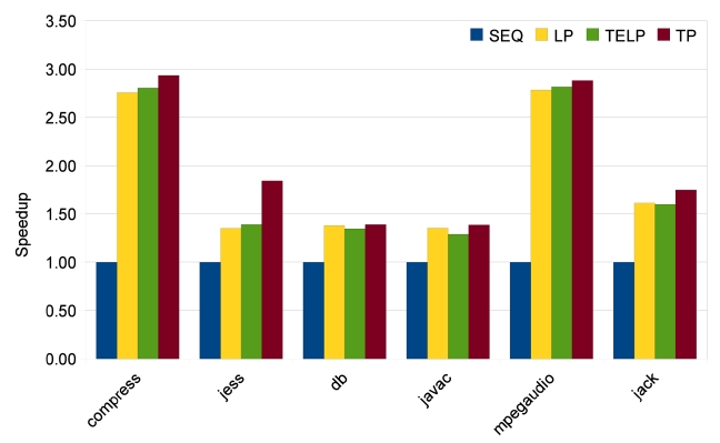
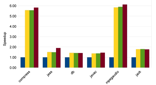
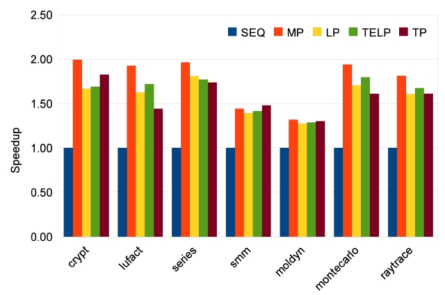
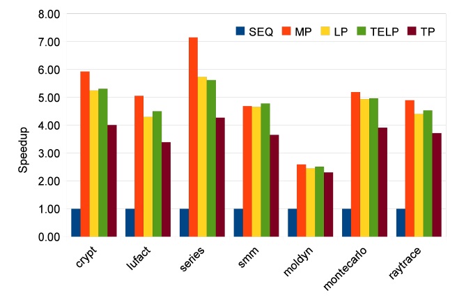
In order to study the scalability of our parallelizing approaches, we measure speedups for 2, 4 and 8 cores. The results of Java Grande benchmarks are shown in Figs. 9-11. The manually parallelized code always has the best speedups, which are 1.77, 3.25, and 5.07 on average. Loop parallelization is close to MP with average speedups at 1.58, 2.86, and 4.53. The results of TELP prove that trace information benefits loop parallelization by providing better average speedups of 1.62, 2.95, and 4.60. However, the scalability of TP is not as good as the other three approaches; its average speedups are 1.57, 2.79, and 3.61, which are close to the others on 2 and 4 cores, but worse than them on 8 cores. The reason is that TP needs a warm-up period to collect enough information
before it can perform a parallelization. We measure the warm-up time by recording the time before the first parallelized method is executed. The data are shown in Fig. 12. It is clear that warm-up times of Java Grande benchmarks take significant portions of the total execution times when the number of cores is increased to 4 and 8. This is because the warm-up time stays constant while the total execution time reduces, especially for the Java Grande benchmarks whose total execution times are short. On the other hand, there is no obvious warm-up time effect on SpecJVM98 benchmarks because of their longer execution times.
The results of SpecJVM98 benchmarks are quite different, as shown in Figs. 13-15. Only two benchmarks, compress and mpegaudio, achieve higher speedups when the number of cores is increased. The other four benchmarks do not show any speedup higher than 2because not all SpecJVM98 benchmarks have good parallelism. We identify the time spent on parallelizable
regions in each benchmark based on trace information, which is shown in Fig. 16. According to Fig. 16, those that achieve satisfying speedups spend at least 70% of their execution times on parallelizable regions, like all benchmarks from Java Grande and the compress and
mpegaudio from SpecJVM98.
The low percentages of parallelizable regions in jess, db, javac and jack explain why their speedups are not good. In some cases like db, heavy loop-carried dependence is the reason for bad parallelism. In some other cases like jess, javac and jack, it is the program structure that prevents sufficient parallelization. However, the TP approach has some strengths in this situation. As shown in Fig. 13, TP achieves much better speedups for jess, javac and jack. Also, TP always achieves the same or better speedups than LP and TELP. This is because TP exploits more parallelism, beyond loop iterations, and at the same time, it also parallelizes loop iterations as duplicated traces. But the parallelism in traces does not have good scalability, as shown in Figs. 14 and 15. Unlike the loop iterations that can be evenly distributed on many cores, only two or three traces may be run in parallel due to data- and control-dependence.
Trace based automatic parallelization has been studied in various works [1, 2]. These orks, however, performs an additional execution to collect trace information off-line, and considers only the simple loop induction/reduction dependency. In contrast, we use on-line trace collection to avoid the expensive profiling execution, and introduce more advanced dependency analysis to deal with more complicated Java programs. In the past two decades, a number of parallelizing compilers have been developed, most of them designed for static high level programming languages, like C and Fortran. Some examples are the SUIF [11] and the Rice dHPF compiler [12]. All these works focused on converting a source code into a high quality parallel executable code. In other words, a source code is required for these approaches. In contrast, our work does not need any source code. Some researches utilized JVM for parallelization. Chan and Abdelrahman [3] proposed an approach for the automatic parallelization of programs that use pointer-based dynamic data structures, written in Java. Tefft and Lee [13] used a Java virtual machine to implement an single instruction multiple data (SIMD) architecture. Zhao et al. [4] developed an online tuning framework over Jikes RVM to parallelize and tune a loop-based program at run-time at acceptable overheads; this framework showed better performance than the traditional parallelization schemes. The core of their work is a loop parallelizing compiler, which detects parallelism among loops, divides loop iterations and creates parallel threads. None of these works, however, uses trace information in their systems.
Another interesting research area is thread-level speculating. Pickett [14] applied speculative multithreading to sequential Java programs in software to speedup existing multiprocessors. Also, Java run-time parallelizing machine (Jrpm), based on a chip multiprocessor (CMP) with threadlevel speculation (TLS) support, [15] is a complete system for parallelizing sequential Java programs automatically. However, speculation always requires additional hardware support. In contrast, our approach is purely software fully implemented inside of Jikes RVM, without any hardware requirement.
In this paper, we have introduced two novel approaches of automatic parallelization for Java programs at runtime. They are pure software-based online parallelization built on a Java virtual machine. Parallelization can be done without any source code or profiling execution. Our experimental results on a 2-core machine indicated good speedup for real-world Java applications that exhibit data-level parallelism. All benchmarks were accelerated and the average speedup was 1.38. While this is less than the ideal speedup on a dual-core processor (i.e., 2), it is not too far away from the speedup of even manually parallelized version of those Java programs, considering that the parallelization is done automatically at run-time by the compiler. Also, we observed a very small overhead, only 0.44% on average, from trace collection and recompilation in our approach. Furthermore, we tested our approaches on 4-core and 8-core processors. Our approaches showed good scalability when there was enough datalevel parallelism in the Java programs. Even for programs that cannot be well parallelized by traditional LP, our second approach, TP, can exploit parallelism beyond loop iterations.