This paper presents novel statistical algorithms for protecting the iTrust information retrieval network against malicious attacks. In iTrust, metadata describing documents, and requests containing keywords, are randomly distributed to multiple participating nodes. The nodes that receive the requests try to match the keywords in the requests with the metadata they hold. If a node finds a match, the matching node returns the URL of the associated information to the requesting node. The requesting node then uses the URL to retrieve the information from the source node. The novel detection algorithm determines empirically the probabilities of the specific number of matches based on the number of responses that the requesting node receives. It also calculates the analytical probabilities of the specific numbers of matches. It compares the observed and the analytical probabilities to estimate the proportion of subverted or non-operational nodes in the iTrust network using a window-based method and the chi-squared statistic. If the detection algorithm determines that some of the nodes in the iTrust network are subverted or non-operational, then the novel defensive adaptation algorithm increases the number of nodes to which the requests are distributed to maintain the same probability of a match when some of the nodes are subverted or non-operational as compared to when all of the nodes are operational. Experimental results substantiate the effectiveness of the detection and defensive adaptation algorithms for protecting the iTrust information retrieval network against malicious attacks.
Modern society depends on the retrieval of information over the Internet. For reasons of efficiency, Internet search and retrieval exploits centralized search engines, and assumes that such search engines are unbiased. Unfortunately, it is easy to enable an Internet search engine to conceal or censor information. History and the present have demonstrated that we cannot depend on centralized search engines to remain unbiased. The moment at which society is most dependent on the free flow of information across the Internet might also be the moment at which information is most likely to be censored or suppressed.
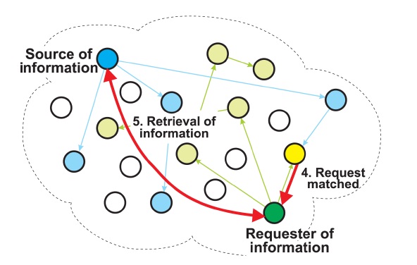
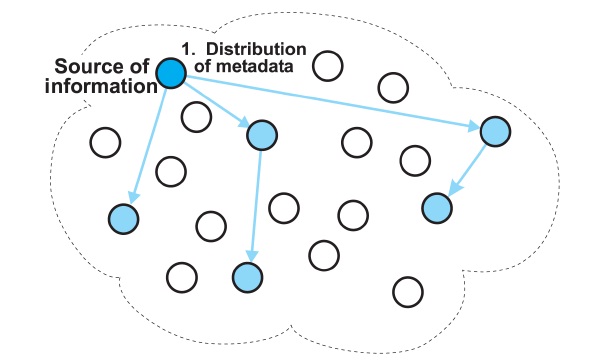
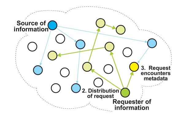
The iTrust system [1,2] is a completely decentralized and distributed information retrieval system, which is designed to defend against the censorship of information on the Internet. In iTrust, metadata describing documents, and requests (queries) containing keywords, are randomly distributed to multiple participating nodes. The nodes that receive the requests attempt to match the key-words in the requests with the metadata they hold. If a node has a match, the matching node returns the URL of the associated information to the requesting node. The requesting node then uses the URL to retrieve the information from the source node.
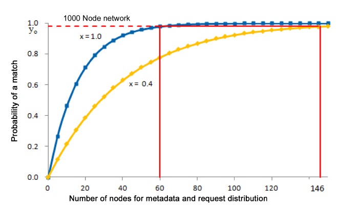
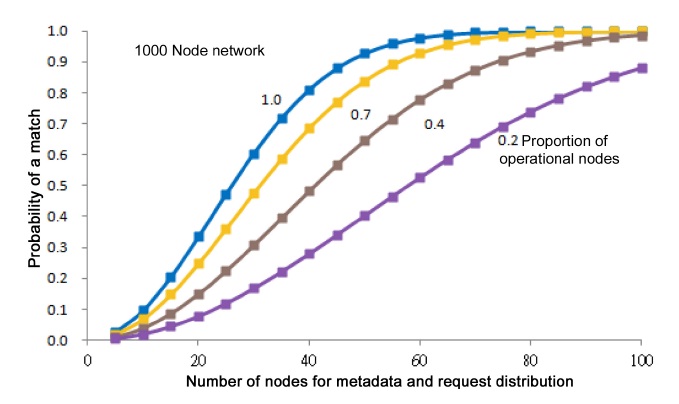
Crucial performance parameters of iTrust are the numbers of nodes to which the metadata and the requests are distributed in order to achieve a high probability of a match. In a network with

nodes results in a probability of a match that exceeds 1 ?
The decentralized and distributed nature of iTrust makes it very robust against malicious attacks that aim to prevent information retrieval. One specific kind of malicious attack is to insert into the network a large number of nodes that behave normally except that they do not match requests and metadata on certain topics. The appropriate response to such an attack is to increase the number of nodes to which the requests are distributed, thus restoring the probability of a match to the desired level. This paper presents novel statistical algorithms for detecting such malicious attacks, using a window-based method and the chi-squared statistic, and for adaptively defending against them by increasing the number of nodes to which the requests are distributed.
The iTrust information retrieval system is completely distributed, and involves no centralized mechanisms and no centralized control. We refer to the nodes that participate in an iTrust network as the
Some nodes, the
Other nodes, the
The participating nodes compare the metadata in the requests they receive with the metadata they hold. If such a node finds a match, which we call an
matching node returns the URL of the associated information to the requesting node. The requesting node then uses the URL to retrieve the information from the source node, as shown in Fig. 3.
The iTrust system runs on laptop, desktop or server nodes on the Internet. There might be hundreds or thousands of iTrust nodes in a typical iTrust network. The primary goal of each iTrust node is to match a query it receives with metadata it holds and to respond with a URL for that resource, if it has a match.
The iTrust implementation on a node consists of the Web server foundation, the application infrastructure, and the public interface. These three components interact with each other in order to distribute metadata and requests and to retrieve resources from the nodes.
The implementation utilizes the Apache Web server along with several hypertext preprocessor (PHP) modules and library extensions. In particular, it uses the standard session and logging modules, and the compiled-in cURL, SQLite, and HTTP PHP extension community library (PECL) modules.
The iTrust system operates over HTTP and, thus, the transmission control protocol/Internet protocol (TCP/IP). As such, it establishes a direct connection between any two nodes that need to communicate; iTrust uses neither flooding nor random walks.
The iTrust system replicates both the metadata and the requests (queries). A source node randomly selects nodes for the distribution of metadata, and a requesting node randomly selects nodes for the distribution of requests. At each node, iTrust maintains a local index of metadata and URLs for the corresponding resources.
When a node receives a request, it compares the metadata (keywords) in the request against a SQLite database consisting of metadata and URLs. If the keywords in the request match locally stored metadata, the node sends a response containing the URL corresponding to the metadata to the requester. When the requester receives the response, it uses the URL in the response to retrieve the information from the source node.
We assume that all of the participating nodes in an iTrust network have the same membership set. Moreover, we assume that the underlying Internet delivers messages reliably and that the nodes have sufficient memory to store the source files and the metadata, which the nodes generate and receive.
The primary parameters determining the performance of the iTrust system are:
n: The number of participating nodes (i.e., the size of the membership set)
x: The proportion of the n participating nodes that are operational (i.e., 1 ? x is the proportion of non-operational nodes)
m: The number of participating nodes to which the metadata are distributed
r: The number of participating nodes to which the requests are distributed
k: The number of participating nodes that report matches to a requesting node.
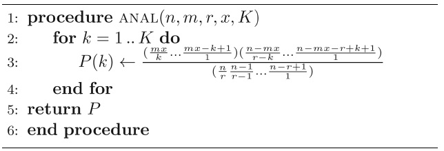
Our probabilistic analysis for iTrust is based on the hypergeometric distribution [4], which describes the number of successes in a sequence of random draws from a finite population without replacement. Thus, it differs from the binomial distribution, which describes the number of successes for random draws with replacement. In iTrust, the probability of
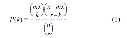
for
Expanding the binomial coefficients in Equation (1), we obtain the following formula for the probability of
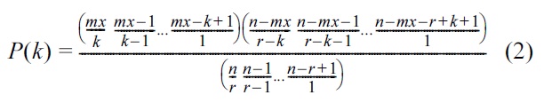
for
For an iTrust network with
The pseudocode for calculating the analytical probabilities from Equation (2) is given in Algorithm 1.
Our algorithm for detecting malicious attacks uses the analytical probabilities given by Algorithm 1 to determine the proportion of nodes in the iTrust network that are operational and, thus, the proportion of nodes that are non-operational or subverted.
[Table10] Algorithm 1 Calculating the analytical probabilities of specific numbers of matches

Algorithm 1 Calculating the analytical probabilities of specific numbers of matches
From Equation (2), we obtain the probability
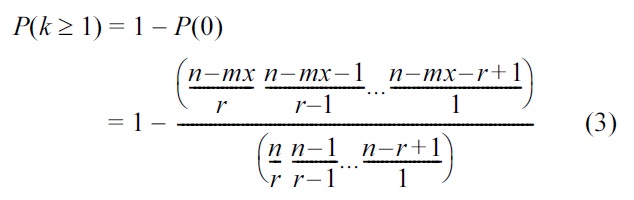
for
For an iTrust network with
Our adaptive algorithm for defending against malicious attacks uses Equation (2) to determine how much to increase the number of nodes to which the requests are distributed to compensate for a decrease in the proportion of operational or non-subverted nodes.
In our experimental studies and in real-world deployments, we cannot use requests that return
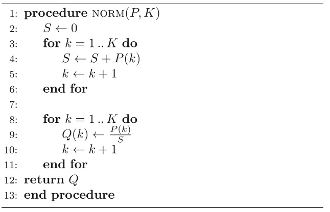
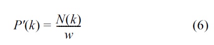
To determine the normalized probabilities
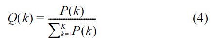
Pseudocode for the normalization method is given in Algorithm 2.
We apply the normalization method given in Algorithm 2 to both the observed probabilities and the analytical probabilities before applying the chi-squared test in the detection algorithm.
[Table11] Algorithm 2 Normalizing the probabilities
Algorithm 2 Normalizing the probabilities
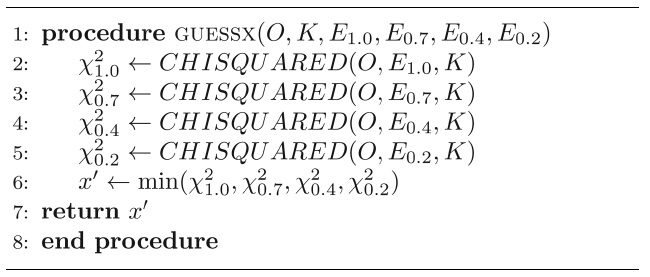
Our detection algorithm uses Pearson’s chi-squared goodness-of-fit test [5] to compare the observed probabilities against the analytical probabilities for different values of
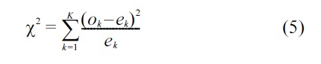
where:
K: The number of buckets into which the observations fall
ok: The actual number of observations that fall into the kth bucket
ek: The expected number of observations for the kth bucket
Pseudocode for the chi-squared method is given in Algorithm 3.
We apply the chi-squared method given in Algorithm 3 in the detection algorithm for estimating
[Table12] Algorithm 3 Computing the chi-squared statistic
Algorithm 3 Computing the chi-squared statistic
V. DETECTION OF MALICIOUS ATTACKS
Our algorithm for detecting malicious attacks first computes the analytical probabilities for the specific numbers of matches for given values of
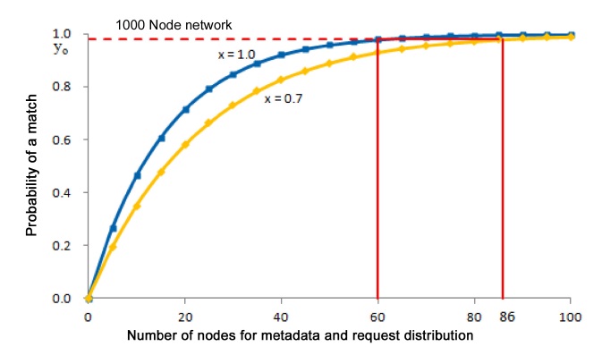
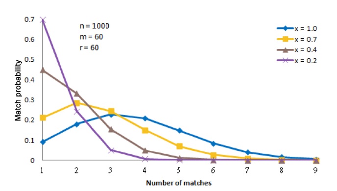
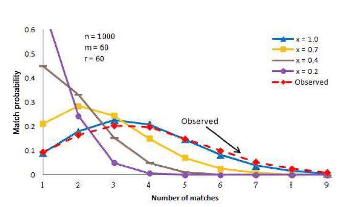
For example, consider an iTrust network with
In Fig. 4, it is easy to distinguish the behavior of the iTrust network with many operational nodes from its behavior with only a few operational nodes. For example, the curves for
The detection algorithm collects statistical data on the number of responses that a requesting node receives for recent requests. Then, it calculates the observed probabilities from the statistical data. The algorithm excludes zero matches (because it cannot distinguish the case in which no node holds both the metadata and the request, and the case in which no such metadata exists). The algorithm then normalizes both the observed probabilities and the analytical probabilities.
Next, it applies the chi-squared statistic in Algorithm 2 to the normalized observed probabilities
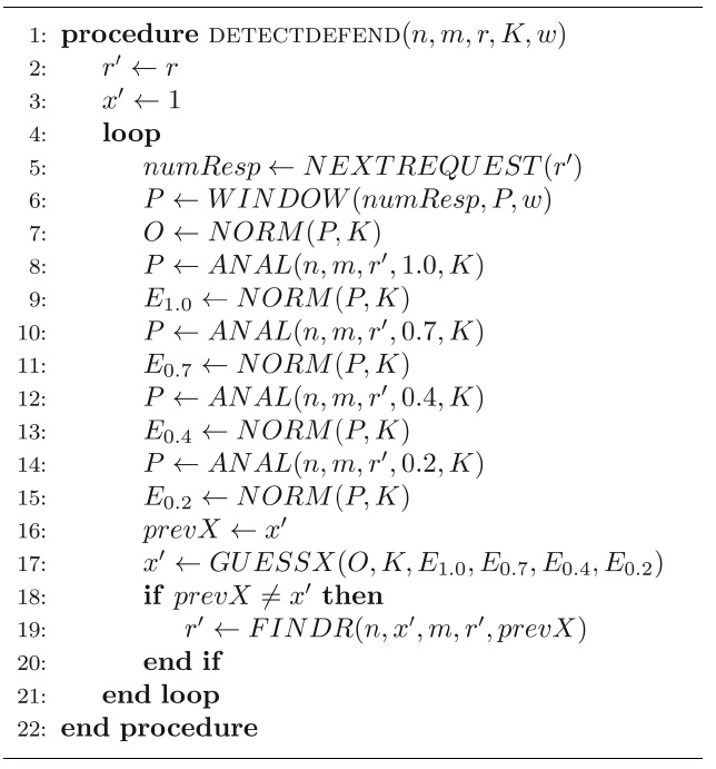
The pseudocode for the detection algorithm is shown in Algorithm 4. Note that the smallest value of the chisquared statistic determines the best estimate of

Algorithm 4 Estimating x' using the chi-squared statistic with the normalized observed probabilities and the normalized analytical probabilities
For example, suppose that the detection algorithm collects the number of matches for each of 3,000 requests, where the proportion of operational nodes is
Next, the detection algorithm applies the chi-squared statistic to calculate the chi-squared value using the normalized observed probabilities and the normalized analytical probabilities for
As illustrated in Fig. 6, based on the 3,000 requests collected, the detection algorithm compares the observed
probabilities against the analytical probabilities for
VI. DEFENSE AGAINST MALICIOUS ATTACKS
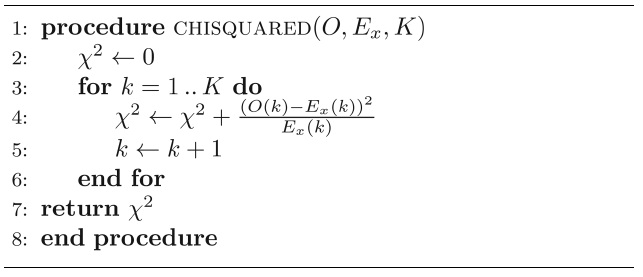
If the detection algorithm determines empirically that the proportion of operational nodes is
Algorithm 5 Iteratively finding the value of r' to maintain a high probability of a match even if some of the nodes are subverted
For example, if the detection algorithm determines empirically that
and
Similarly, in Fig. 8, if the detection algorithm determines empirically that
In order to evaluate the ability of the detection algorithm to estimate the proportion
We use libCURL (which is a free client-side URL transfer library for transferring data using various protocols) to collect the number of responses (matches). We randomly select nodes without repetition from the membership set for distribution of the metadata and the requests.
Before we start the emulation program, we initialize the values of
>
A. Parameters of the Detection Algorithm
The primary parameters that we investigate for the detection algorithm are defined below:
K: An upper bound on the number k of responses to requests, i.e., an upper bound on the number of buckets used for the responses. Note that, from Equation (2), K ≤ min{mx, r}.
t: The number of chi-squared evaluations that indicate the same change in the value of x' before action is taken to change the value of r'.
s: The number of requests for which responses are accumulated before the chi-squared statistic is calculated
w: The number of recent requests that are used in the calculation of chi-squared. For example, for w = 10, we use the current request i, the previous request i ? 1, ..., back to the 9th request i ? 9 in the calculation of chisquared.
>
B. Ranges for the Experimental Evaluation
Initially, we collected 10,000 requests from the emulation program with
By definition, accuracy is the number of correct estimates of
To determine the accuracy of the detection algorithm, for each value of
For each request in the window, the algorithm determines the number of responses the requester received for that request. To determine the observed probability
and then normalizes
From the analytical formula (2), the algorithm calculates
The algorithm then computes the chi-squared statistic using Algorithm 3 with the normalized
In our experiments, we consider windows of sizes
We repeat the same process 100 times and average the results to obtain the final accuracy
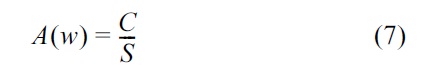
The response time represents the number of responses before the detection algorithm determines a change in the estimated value of
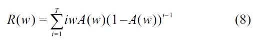
In Equation (8), the probability that the value of
Simplifying Equation (8), we obtain:
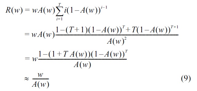
The response time, in seconds, depends not only on the number of requests in the window but also on the time interval between requests, i.e., the time between issuing a request and obtaining the responses for that request plus the time to create and issue the request (think time). If it takes
In our window-based algorithm, the requester issues requests, collects responses, and determines the observed probabilities based on the responses to the
>
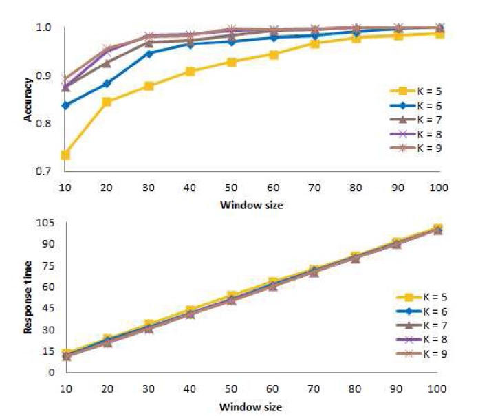
A. Determining an Appropriate Value of K
For the window-based algorithm and the chi-squared statistic, first we consider the number
[Table.15] Algorithm 6 Window-based algorithm
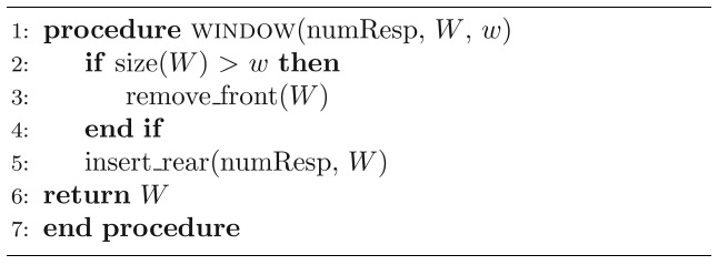
Algorithm 6 Window-based algorithm
Fig. 9 presents the mean accuracy at the top of the figure, and the mean response time at the bottom of the figure, as a function of the window size. In the figure, we see that the accuracy for
Based on these results, for
>
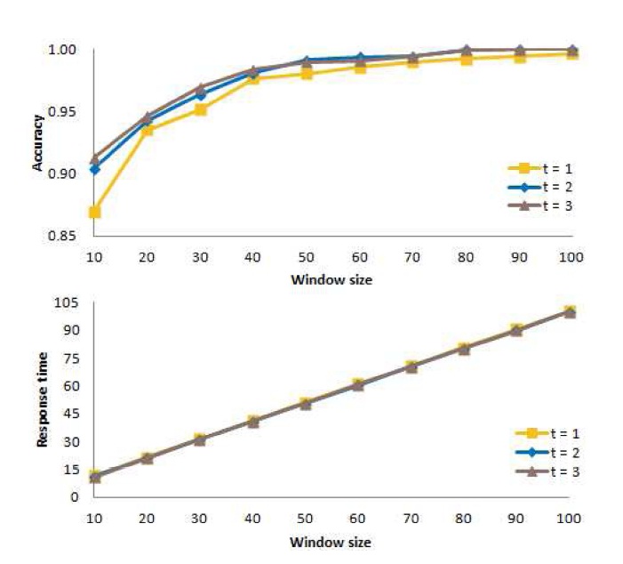
B. Determining an Appropriate Value of t
Next, for the window-based algorithm, we consider the number
In these experiments, we consider three different values of
change in the value of
Fig. 10 shows the mean accuracy at the top of the figure, and the mean response time at the bottom of the figure when action is taken immediately (
Thus, from our experiments, we conclude that
>
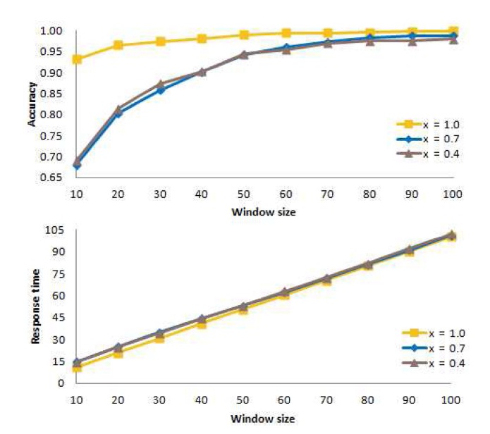
C. Determining an Appropriate Value of s
Now, for the window-based algorithm, we consider the number
of
In these experiments, we consider three different values of
Fig. 11 shows the mean accuracy at the top of the figure and the mean response time at the bottom of the figure when action is taken immediately (
From these experiments, we conclude that
>
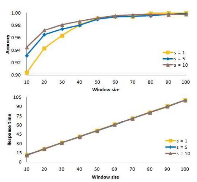
D. Determining an Appropriate Value of w
Fig. 12 shows the mean accuracy at the top of the figure and the mean response time at the bottom of the figure, as a function of the window size
The figure illustrates that the accuracy values for
50, the accuracy values for all values of
Ideally, the accuracy should be high, and the response time should be low. However, when we compare the top curve and the bottom curve for specific values of
X. COMBINING DETECTION AND DEFENSE
The pseudocode for the combined algorithms is shown in Algorithm 7.
In lines 2 and 3, the variables are initialized. Line 4 begins a loop that repeats indefinitely until there are no more requests. Within the loop, in line 5, the requester issues a request based on
In line 6, the algorithm calculates the current observed
[Table.16] Algorithm 7 Combined detection and defensive adaptation algorithms

Algorithm 7 Combined detection and defensive adaptation algorithms
analytical probabilities and normalizes them to obtain the normalized analytical probabilities
In line 17, the algorithm estimates the value of
In line 18, the algorithm compares
Then, the algorithm goes back to line 5 to acquire another request based on the value of
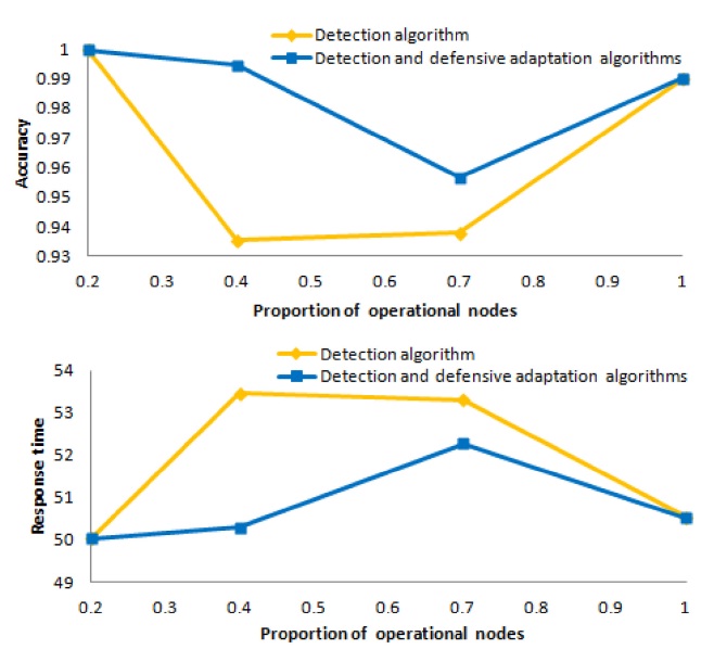
Now, we compare the mean accuracy and the mean response time for the detection algorithm against the mean accuracy and the mean response time for the combined detection and defensive adaptation algorithms for
For these experiments, we set
Fig. 13 shows the mean accuracy at the top of the figure and the mean response time at the bottom of the figure, for the detection algorithm and the combined detection and defensive adaptation algorithms as a function of
At the top of the figure, the light (yellow) curve shows the accuracy of the results obtained from the detection algorithm, and the dark (blue) curve shows the accuracy
of the results obtained from the combined detection and defensive adaptation algorithms. We see that the accuracy for
Similarly, at the bottom of the figure, the light (yellow) curve shows the response time for the detection algorithm, and the dark (blue) curve shows the response time for the combined detection and defensive adaptation algorithms. We observe that, when we use the combined detection and defensive adaptation algorithms, the response time decreases substantially for both
Overall, these experiments demonstrate that the detection algorithm is effective in discovering that the iTrust network contains non-operational or subverted nodes, and that false alarms rarely occur. Furthermore, the defensive adaptation algorithm is effective in defending against malicious attacks, because it appropriately adjusts the number of nodes to which the requests are distributed in order to maintain a high probability of a match. By selecting appropriate values of the parameters, and by using the combined algorithms, we obtain high accuracy and reasonable response time.
Peer-to-peer networks have been characterized as structured or unstructured [6]. The structured approach requires the nodes to be organized in an overlay network, based on a distributed hash table, tree, ring, etc. The unstructured approach uses randomization and/or gossiping to distribute the metadata (or data) and the requests to nodes in the network. The iTrust system uses the unstructured approach.
Gnutella [7], one of the first unstructured peer-to-peer networks, uses flooding of requests. A node makes a copy of a file when it receives the file it requested. If the query rate is high, nodes quickly become overloaded and the system ceases to function satisfactorily. To address this problem, Ferreira et al. [8] use random walks, instead of flooding, to replicate objects and propagate queries. Gia [9] employs biased random walks to direct queries towards high-capacity nodes. iTrust does not use flooding or random walks, but rather distributes the metadata and the requests to nodes chosen uniformly at random.
Freenet [10] replicates an object at a node, even though the node did not request it. Nodes that successfully respond to requests receive more metadata and more requests, making it easy for a group of untrustworthy nodes to gather most of the searches into their group. Likewise, the adaptive probabilistic search (APS) method [11] uses feedback from previous searches to direct future searches, instead of distributing the requests uniformly at random, like iTrust does.
Cohen and Shenker [12] show that square root replication is theoretically optimal for minimizing the search traffic. They replicate objects based on the access frequencies (popularities) of the objects. Lv et al. [13] also use square root replication, and adaptively adjust the replication degree based on the query rate. iTrust likewise exploits square root replication but distributes the metadata uniformly at random, so that popular nodes are not more vulnerable to attack.
BubbleStorm [14] replicates both queries and data, hybridizes random walks and flooding, and considers churn, joins, leaves and crashes. Leng et al. [15] present mechanisms for maintaining the desired degree of replication in BubbleStorm, when each object has a maintainer node. In iTrust, we use different techniques to maintain the desired degree of replication of the metadata and the requests.
PlanetP [16] maintains a local index that contains metadata for documents published locally by a peer. Similarly, iTrust maintains a local index of metadata and corresponding URLs for the data. PlanetP also uses a global index that describes all peers and their metadata in a Bloom filter, which it replicates throughout the network using gossiping. GALANX [17] directs user queries to relevant nodes by consulting a local peer index. Like iTrust, GALANX is based on the Apache HTTP Web server.
Morselli et al. [18] describe an adaptive replication protocol with a feedback mechanism that adjusts the number of replicas according to the mean search length, so that an object is replicated sufficiently. Their adaptive replication protocol is quite different from the defensive adaptation algorithm of iTrust.
Sarshar et al. [19] use random walks and bond percolation in power law networks with high-degree nodes. The high-degree nodes in such networks are subject to overloading and are vulnerable to targeted malicious attacks. They note that “protocols for identifying or compensating for such attacks, or even recovering after such an attack has disrupted the network are yet to be designed.” We present such protocols in this paper.
Jesi et al. [20] identify malicious nodes in a random overlay network based on gossiping and put such nodes on a blacklist. They focus, in particular, on hub attacks in which colluding malicious nodes partition the network by spreading false rumors. iTrust does not use gossiping but, rather, uses random distribution of the metadata and the requests and, thus, is less subject to hub attacks.
Condie et al. [21] present a protocol for finding adaptive peer-to-peer topologies that protect against malicious peers that upload corrupt, inauthentic or misnamed content. Peers improve the trustworthiness of the network by forming connections, based on local trust scores defined by past interactions. Effectively, their protocol disconnects malicious peers and moves them to the edge of the network.
Several network security researchers use the chisquared statistic in their work. In particular, Goonatilake et al. [22] apply the chi-squared statistic to intrusion detection. We also use the chi-squared statistic in the detection algorithm of iTrust.
XII. CONCLUSIONS AND FUTURE WORK
We have presented novel statistical algorithms for protecting the iTrust information retrieval network against malicious attacks. The detection algorithm determines empirically the probabilities of specific numbers of matches based on the number of responses that a requesting node receives. Then, it compares the normalized observed probabilities with the normalized analytical probabilities for specific numbers of matches, to estimate the proportion of nodes that are operational, using a window- based method and the chi-squared statistic. If some of the nodes are subverted or non-operational, the defensive adaptation algorithm increases the number of nodes to which the requests are distributed to maintain the same probability of a match as when all of the nodes are operational. By selecting appropriate values of the parameters, and by using the combined detection and defensive adaptation algorithms, we obtain high accuracy and reasonable response time. In the future, we plan to investigate other kinds of malicious attacks on iTrust, as well as algorithms for protecting iTrust against those kinds of malicious attacks.