In databases, keys play a fundamental role in understanding both the structure and semantics. Given an SQL table schema, a key is a collection of columns whose values uniquely identify rows. That is, no two different rows have matching total values in each of the key columns. The concept of a key is essential for many other data models, including semantic models [1-4], object models [5], description logics [6], XML [7-9], RDF [10], and OWL [11].
The discovery of semantically meaningful SQL keys is a crucial task in many areas of modern data management, for example, in data modeling, database design, query optimization, indexing, and data integration [12]. This article is concerned with methods for semi-automated schemadriven and automated data-driven SQL key discovery.
There is great demand in industry for such methods, because they vastly simplify the job of the database administrator and thereby decrease the overall cost of database ownership. The discovery of composite keys is especially difficult, because the number of possible keys
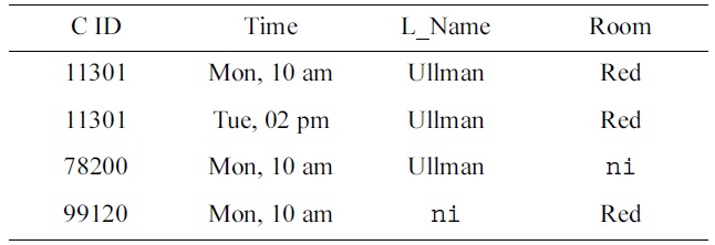
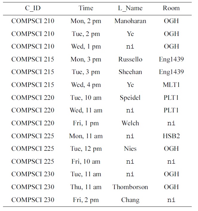
[Table 1.] An Armstrong table for SCHEDULE
An Armstrong table for SCHEDULE
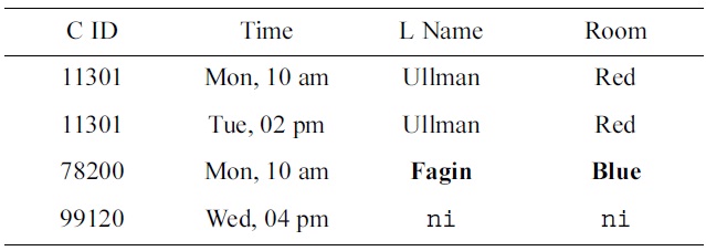
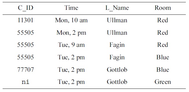
[Table 2.] Another Armstrong table

Another Armstrong table
increases exponentially with the number of columns [3,13]. Because of the industry demand, the goal is to provide practical algorithms that exhibit good typical case behavior. Industry-leading data modeling and design tools, such as the
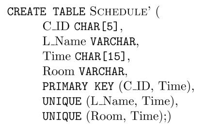
Consider a simple database that collects basic information about the weekly schedule of courses. That is, we have a schema SCHEDULE with columns
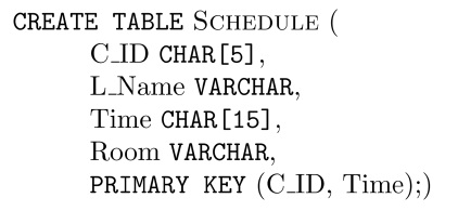
The table schema specifies additional assertions. The primary key forces rows over SCHEDULE to be NOT NULL in the

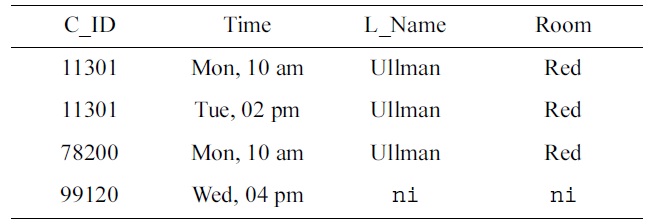
Updated table
their {
The domain experts express concern about rows 1 and 3: Ullman teaches both 11301 and 78200 in the red room on Monday at 10 am. After some discussion, the domain experts emphasize that different courses should not be taught by the same lecturer in the same room at the same time. As a consequence, the team of engineers decides to specify the uniqueness constraint (UC)
The domain experts direct the engineers’ attention to rows 1 and 3 where Ullman teaches both 11301 and 78200 on Monday at 10 am. After exchanging some ideas, the experts agree that lecturers must not teach different courses at the same time.
Moreover, from rows 1 and 4 of the data sample in Table 2, experts notice that both 11301 and 78200 are taught on Monday at 10am in the red room. It turns out that no two different courses must be taught at the same time in the same room. Therefore, the UC
While this approach appears to be very beneficial, the question remains what constitutes good test data, and how to create it (automatically). In some situations the domain experts may feel very confident and would like to have the opportunity to modify values in the test data to reflect their domain knowledge, or provide the entire test data themselves. In such cases, and other situations, the data engineers require automated means to discover a representation of the keys that are satisfied by the test data. For example, when the domain experts inspect the data sample in Table 1, they may simply suggest using the data sample in Table 3 instead, with the updated values indicated by bold font.
On input of this table, a constraint mining algorithm would return NOT NULL constraints on
In this paper we will establish detailed answers to the two questions above. As our first main contribution we discuss the schema-driven discovery of SQL keys that are semantically meaningful for a given application domain. For this purpose we investigate the well-known concept of Armstrong databases for the class of SQL keys. Armstrong databases formalize the concept of good test data in the sense that they satisfy the set Σ of keys currently perceived as semantically meaningful, and violate all keys that are not implied by Σ. We characterize when a given SQL table is Armstrong with respect to a given set Σ of SQL keys. This characterization allows us to establish an algorithm that generates good test data for arbitrary sets of SQL keys. While we demonstrate that the problem of computing such Armstrong tables is precisely exponential in the number of column headers, our algorithm produces an Armstrong table whose size is at most quadratic. We also show that there are situations where the size of the Armstrong table our algorithm produces is exponentially smaller than the size of the keys given. Both extreme cases result from very specific situations, which are very unlikely to occur in practice. Indeed, in most situations that do occur in practice, our algorithm will produce Armstrong tables whose size is in the same order of magnitude as the size of the keys given.
As a second main contribution we discuss the datadriven discovery of SQL keys. For this purpose we establish two algorithms that compute the set of minimal SQL keys satisfied by a given SQL table. While the problem generally requires exponential time, our algorithms show good best case behavior. As a third main contribution we combine the schema-driven and data-driven approach to increase the effectiveness of SQL key discovery. Given a real world data set, we apply the data-driven approach to identify the minimal SQL keys satisfied by this data set, and then apply the schema-driven approach to compute an Armstrong table for the set of these minimal keys. The Armstrong table is called informative as it contains only rows of the original data set, is much smaller in size, and satisfies the same SQL keys.
As the final contribution, we define formal measures that can be applied to 1) empirically validate the usefulness of our Armstrong tables for the acquisition of semantically meaningful SQL keys, and 2) automate the feedback and marking of database exam questions.
We summarize related work in Section II, and provide preliminary definitions in Section III. We investigate structural and computational properties of Armstrong tables for the class of SQL keys in Section IV. In Section V we study the SQL key mining problem. Section VI combines the data-driven and schema-driven approaches to the discovery of SQL keys. Our formal measures of usefulness and their applications are discussed in Section VII. Finally, in Section VIII, we conclude and briefly comment on future work.
Data dependencies have been studied thoroughly in the relational model of data, cf. [15-17]. Dependencies are essential to the design of the target database, the maintenance of the database during its lifetime, and all major data processing tasks [15,17]. These applications also provide strong motivation for developing data mining algorithms to discover the data dependencies that are satisfied by a given database. Armstrong databases are a useful design aid for data engineers, which can help with the consolidation of data dependencies [18,19] and schema mappings [20], the design of databases [21] and the creation of concise test data [22].
In the relational model of data, the class of keys is subsumed by the class of functional dependencies. The structural and computational properties of Armstrong relations have been investigated in the relational model of data for the class of keys [3,23], and the more general class of functional dependencies [21,24]. The mining of keys and functional dependencies in relations has also received considerable attention in the relational model [12,25,26]. The concept of informative Armstrong databases was introduced in [22] as semantic samples of existing databases.
One of the most important extensions of Codd’s basic relational model [27] is incomplete information [28,29]. This is mainly due to the high demand for the correct handling of such information in real-world applications. Approaches to deal with incomplete information comprise incomplete relations, or-relations or fuzzy relations. In this paper we focus on incomplete bags, and the most popular interpretation of a null marker as “no information” [29,30]. This is the general case of SQL tables where duplicate rows and null markers are permitted to occur in columns that are specified as null-able. Relations are idealized special SQL tables where no duplicate rows can occur and all columns are specified NOT NULL. Recently, Armstrong tables have been investigated for their combined class of SQL keys and functional dependencies [31]. In this article, we establish optimizations that arise from the focus on the sole class of SQL keys. This provides insight into the trade-off between the expressiveness of data dependency classes and the structural and computational properties of Armstrong tables. The insight can be used by data engineers to make a more informed decision about the complexity of the design process for the target database. For example, it may appear that the most important requirements of an application domain can already be captured by SQL keys alone, without the need for functional dependencies. In this case, engineers can utilize the algorithms developed in the current article, which result in computations that are more resource-efficient than those developed for the combined class of keys and functional dependencies [31]. Note that Hartmann et al. [1] studies Codd keys, which require tuples to have unique and total projections on key attributes. In contrast, the present article studies SQL keys, which require total tuples to have unique projections on key attributes. Hartmann et al. [1] does also not discuss any key mining algorithms or measures to assess the difference of key sets, nor does it discuss informative Armstrong databases. To the best of the authors’ knowledge, no previous work has addressed the mining of keys from SQL tables. Our results reveal that the methods developed for the idealized special case of relations [26] can be adapted to the use for SQL tables. We are also unaware of any studies related to informative Armstrong databases except [22], measures that capture the difference between sets of keys, nor their utilization for assessing the usefulness of Armstrong tables or database exam questions.
The present article is an extension of the conference paper [32]. The present article contains all the proofs of our results as well as additional motivation and discussion. In addition, the concept of informative Armstrong tables was not discussed in the conference paper.
In this section we introduce the basic definitions necessary and sufficient for the development of our results in subsequent sections. In particular, we introduce a model that is very similar to SQL’s data definition capabilities. The interpretation of null marker occurrences as “no information” follows the SQL interpretation, and the formal model introduced by Zaniolo [29]. The class of SQL keys under consideration is the exact class of uniqueness constraints defined in the SQL standard [33].
Let
be a countably infinite set of symbols, called

Each header
For header sets
A UC over a table schema
Following Atzeni and Morfuni [30] a
In schema design and maintenance data dependencies are normally specified as semantic constraints on the tables intended to be instances of the schema. During the design process or the lifetime of a database one usually needs to determine further dependencies, which are implied by the given ones. Let
THEOREM 1.
For the reverse direction we present the contraposition. That is, we assume that for all

and show that under this assumption Σ does not imply
that is,
Again, the construction ensures that
In the relational model of data, keys enjoy a simple axiomatization [17] by two axioms. The set axiom says that for every relation schema
EXAMPLE 1. We can capture the SQL table schema of the running example as the table schema SCHEDULE =
IV. SCHEMA-DRIVEN SQL KEY DISCOVERY
In this section we investigate the structural and computational properties of suitable data to test the semantic meaningfulness of uniqueness constraints over the SQL table schemata. For this purpose, we use Armstrong tables to formalize the notion of suitable test data. Having introduced the concepts of strong agree sets and anti-keys, we characterize when an arbitrarily given SQL table is Armstrong for an arbitrarily given set of uniqueness constraints. The characterization is then used to compute Armstrong tables. Finally, we derive results on the time and space complexity associated with the computation of Armstrong tables.
The official concept of an Armstrong database was originally introduced by Fagin [16]. We require our tables to be Armstrong with respect to uniqueness constraints and the NFS. Intuitively, an Armstrong table satisfies the given constraints and violates the constraints in the given class that are not implied by the given constraints. This results in the following definition.
DEFINITION 1.
Through the use of Theorem 1, it is easy to see that a table
EXAMPLE 2. Let SCHEDULE =
A natural question to ask is how we can characterize the structure of tables that are Armstrong. With this in mind, we introduce the formal notion of strong agree sets for pairs of distinct rows, and tables.
DEFINITION 2.
EXAMPLE 3. Let SCHEDULE =
For a table
DEFINITION 3.
Hence, an anti-key for Σ is given by a maximal set of column headers, which does not form a uniqueness constraint implied by Σ.
EXAMPLE 4. Let SCHEDULE =
>
B. Structure of Armstrong Tables
The concepts from the last sub-section are sufficient to establish a characterization of Armstrong tables for the class of UCs over SQL table schemata.
THEOREM 2.

Proof. First, we show that the three conditions are sufficient for
Showing that the three conditions hold necessarily whenever
EXAMPLE 5. Let SCHEDULE =
>
C. Computation of Armstrong Tables
We will now use the characterization of Theorem 2 to compute Armstrong tables for an arbitrarily given set Σ of UCs and an arbitrarily given NFS
LEMMA 1.

We show first that if
This, however, contradicts the minimality of
Now, we show that if
From
That is,
Now, we have a complete strategy for computing Armstrong tables, which we summarize in Algorithm 1. For each column header

saying that a table can have at most one row. Here, we just need to return a table consisting of one row with null marker occurrences in columns which are null-able. Otherwise, we start off with a row
[Algorithm1] Algorithm 1 Armstrong table computation
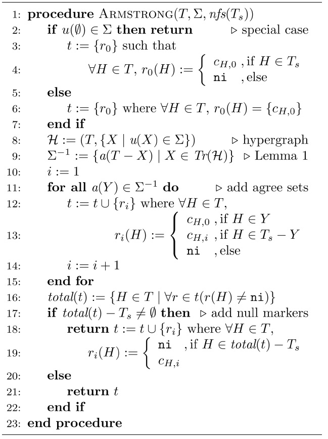
Algorithm 1 Armstrong table computation
The correctness of Algorithm 1 follows from Lemma 1 and Theorem 2.
THEOREM 3.
EXAMPLE 6. Let SCHEDULE = CTLR with SCHEDULE
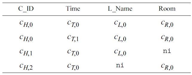
A suitable value substitution yields the data sample in Table 2. □
>
D. Complexity Considerations
In this subsection, we investigate properties regarding the space and time complexity for computing Armstrong tables. We will demonstrate that the user-friendly representation of a set of SQL keys in the form of an Armstrong table comes, in the worst case, at a price. In fact, the number of rows in a minimum-sized Armstrong table can be exponential in the total number of column headers that occur in Σ. Because of this result we cannot, in the worst case, design an algorithm for generating Armstrong tables in polynomial time.
1) Worst-case time-complexity
The following result follows straight from Theorem 2 and the correctness of Algorithm 1.
PROPOSITION 1.
Finally,
since every distinct pair of distinct tuples in
Let the size of an Armstrong table be defined as the number of rows that it contains. It is a practical question to ask how many rows a minimum-sized Armstrong table requires. An Armstrong table
We recall what we mean by
PROPOSITION 2.
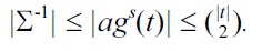
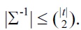
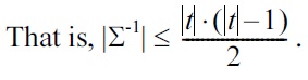
It remains to show that there is a set Σ of UCs for which the number of rows in each Armstrong table for Σ is exponential in the size of the UCs given. According to Theorem 1 it suffices to find a set Σ of UCs such that Σ-1 is exponential in the size of the UCs. Such a set is given by
Σ = {u(H2i-1, H2i) | i = 1, . . . , n}.
The set Σ-1 consists of those anti-keys that contain precisely one column header for each element of Σ. Therefore, Σ-1 contains precisely 2
2) Minimum-sized Armstrong tables
Despite the general worst-case exponential complexity in the size of the keys, Algorithm 1 is a fairly simple algorithm that is, as we now demonstrate, quite conservative in its use of time.
PROPOSITION 3.
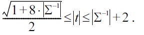
Consequently,
□
Note the upper bound in Proposition 3. In general, the focus on UCs can yield Armstrong tables with a substantially smaller number of rows than Armstrong tables for more expressive classes such as functional dependencies. The reason is that we do not need to violate any functional dependencies that are not implied by the given set. In practice, this is desirable for the validation of schemata known to be in Boyce-Codd normal form, for example. Such schemata are often the result of entity-relationship modeling. Applying the algorithm from [31], designed for UCs and functional dependencies, to our running example would yield an Armstrong table with 12 rows. Instead, Algorithm 1, designed for UCs only, produces an Armstrong table with just 4 rows. In general, we can conclude that Algorithm 1 always computes an Armstrong table of reasonably small size.
COROLLARY 1.
3) Size of representations
We show that, in general, there is no superior way of representing the information inherent in a set of UCs and a null-free subschema.
THEOREM 4.
For the second claim let
We can perceive that the representation in form of an Armstrong table can offer tremendous space savings over the representation as a UC set, and vice versa. It seems intuitive to use the representation as Armstrong tables for the discovery of semantically meaningful constraints, and the representation as constraint sets for the discovery of semantically meaningless constraints. This intuition has been confirmed empirically for the class of functional dependencies over relations [18].
V. DATA-DRIVEN SQL KEY DISCOVERY
In this section we will establish algorithms for the automated discovery of uniqueness constraints from given SQL tables. Such algorithms have direct applications in schema design, query optimization, and the semantic sampling of databases [22,26,31,36,37]. In requirements engineering, for example, these algorithms can be utilized to discover semantically meaningful uniqueness constraints from sample data, which domain experts provide.
>
A. Mining by Pairwise Comparison of Rows
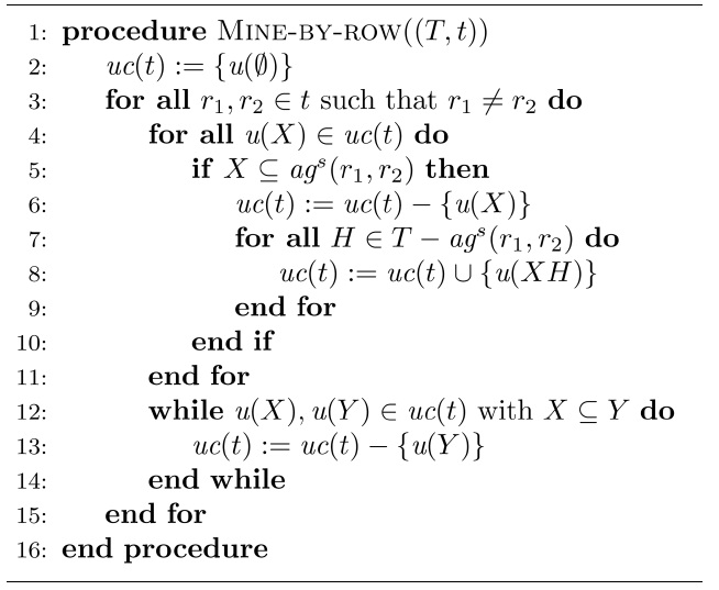
Our first algorithm gradually inspects all pairs of rows for the given table, and adjusts the set of minimal UCs accordingly. More specifically, for every given pair of different rows
whenever
[Algorithm2] Algorithm 2 Mining of uniqueness constraints by pairwise row comparisons

Algorithm 2 Mining of uniqueness constraints by pairwise row comparisons
THEOREM 5.
For the complexity bound note that there are |
EXAMPLE 7. Let
The UCs are those explained in the introductory section of this article. □
>
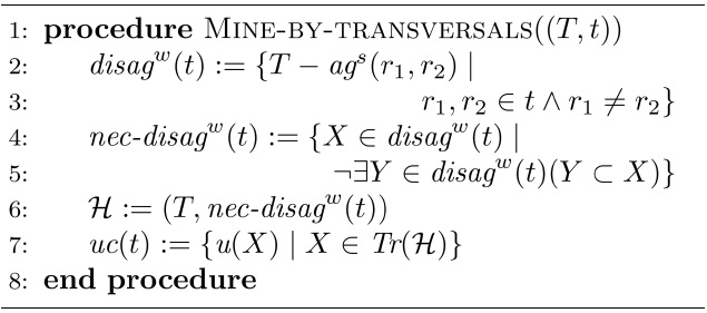
B. Mining by Exploration of Hyper-Graph Transversals
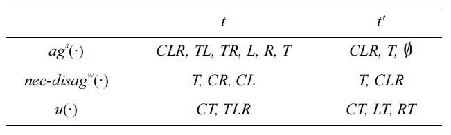
Again, our next algorithm uses the concept of hypergraph transversals. Indeed Algorithm 3 computes the complements of the strong agree sets for the given input table (lines 2 and 3). These complements are called weak disagree sets. Lines 4 and 5 compute the necessary weak disagree sets, that is, those weak agree sets that are minimal. For the hypergraph where the node set is
The following lemma explains the soundness of Algorithm 3.
LEMMA 2.
[Algorithm3] Algorithm 3 Mining of uniqueness constraints by exploring hypergraph transversals

Algorithm 3 Mining of uniqueness constraints by exploring hypergraph transversals
First, if
and there would be some
which contradicts the hypothesis that
This, however, would violate the minimality of
Now, we demonstrate that the two conditions are sufficient for
From |≠
holds. Consequently, for all
We conclude that
THEOREM 6.
The collection
EXAMPLE 8. Let
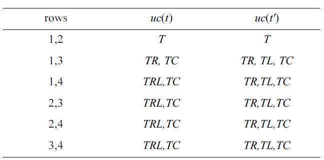
The next table shows the steps for applying Algorithm 3 to (SCHEDULE,
The UCs are those explained in the introductory section of this article. □
VI. INFORMATIVE ARMSTRONG TABLES
Here, we combine the schema- and data-driven approach to the discovery of SQL keys, as given in Sections IV and V, respectively. The disadvantage of the schema-driven approach is that the Armstrong tables, when generated by our algorithm, contain only artificial values. It is therefore doubtful that such tables illustrate the current perceptions of the data engineers to the domain experts who inspect the table. Of course, the data engineers may substitute real domain values for the artificial values before they present the table to the domain experts, or they generate the Armstrong tables on the basis of some real domain values. However, the table may still not be a good representative of the real world application domain, since some of the combinations of the values may never occur in practice. We will now outline a solution to this problem, which overcomes this limitation. Here, the assumption that is necessary is that some real world data set t is available, for example, in the form of legacy data. Under this assumption, we can apply the data-driven algorithms from Section V to mine the set
[Table 4.] Real-world table treal

Real-world table treal
[Table 5.] Informative Armstrong table tinf for treal
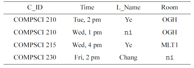
Informative Armstrong table tinf for treal
DEFINITION 4.
In the context of this paper, we are interested in informative Armstrong tables with respect to the class
The data sample
{u(Time), u(C_ID,L_Name), u(Room,L_Name)}.
It is not difficult to compute the maximal null-free subschema
{a(L_Name), a(C_ID,Room)}.
Now, finding rows in
VII. EMPIRICAL MEASURES OF USEFULNESS
In this section we describe how the usefulness of applying Armstrong tables for the discovery of semantically meaningful SQL keys can be measured. For this purpose, we will first introduce different measures of usefulness, and then describe a detailed example illustrating how the marking and feedback for non-multiple choice questions in database courses can be automated.
>
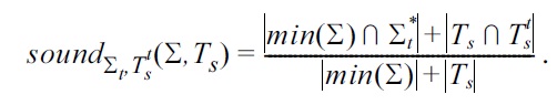
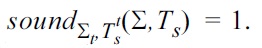
A. Soundness, Completeness, and Proximity
Measuring the usefulness of applying Armstrong tables for the discovery of semantically meaningful SQL keys appears to be non-trivial. However, one may conduct a two-phase experiment where database design teams are given an application domain and are asked to specify the set of UCs they perceive as semantically meaningful. In the first phase, they are not given any help, except natural language descriptions by domain experts. In the second phase, our algorithm can be used to produce Armstrong tables for the set of UCs the teams perceive currently as semantically meaningful. The Armstrong tables may be inspected together with the domain experts, and when new UCs are identified a corresponding Armstrong table may be repeatedly produced. For an experiment or assignment, one may specify a target set Σ
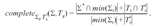
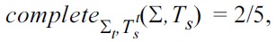
If

and

we define
[Table 6.] Armstrong table as feedback

Armstrong table as feedback
cally meaningful (minimal) UCs and headers in NFSs, are currently perceived as semantically meaningful:
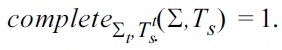
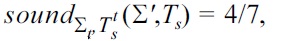
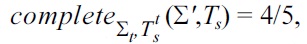
If

and

we define
Finally,
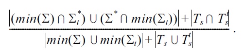
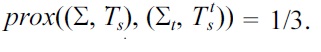
If
and
we define
In database courses one may use Armstrong tables as automated feedback to solutions. Our measures can be applied to automatically mark non-multiple choice questions. This can reduce errors and save time in assessing course work.
Again, we will use our running example where SCHEDULE consists of the four attributes C(_ID), L(_Name), R(oom), and T(ime). Suppose we describe, in natural language, the application domain to the students of a database course. Then, we ask them to identify the uniqueness and NOT NULL constraints that they perceive to be semantically meaningful for this application domain. The students may ask questions in natural language to clarify their perceptions about the application domain. The lecturers of the course act as domain experts who will provide answers to questions in natural language that are consistent with the target set Σ
over the table schema SCHEDULE.
Suppose one group of students returns as an answer to the question the set Σ = {
and
Furthermore, one may also return an Armstrong table for Σ and
The students inspect the table and may make several observations. For example, Fagin teaches 55505 and Gottlob teaches 77707 at the same time in the same room. The students decide to ask the domain expert whether different courses can be taught in the same room at the same time. The domain experts indicate that this is impossible, and the students decide to replace the UC
and
Hence, inspecting the Armstrong table results in an improvement of 1/14 in soundness, 2/5 in completeness, and 1/6 in proximity.
VIII. CONCLUSION AND FUTURE WORK
We investigated the data- and schema-driven discovery of SQL keys. We established insights into structural and computational properties of Armstrong tables. These can increase the discovery of semantically meaningful SQL keys in practice, leading to better schema designs and improved data processing. In addition, we also established algorithms to automatically discover SQL keys in given SQL tables. These have applications in requirement acquisition, schema design and query optimization. We combined the data- and schema-driven approaches to compute informative Armstrong tables, which are effective semantic samples of given data sets. Moreover, we defined formal measures to assess the difference between sets of SQL keys. These can be applied to validate the usefulness of Armstrong tables and to database education. Our findings also apply to Codd’s null marker interpretation