An image is composed of a number of regions that contain background, foreground, textures, and meaningful objects. In other words, an image is a set of attention objects (AO) that capture the user’s attention and interests. For example, human-related objects, such as a human face, a flower, a house, or a text sentence, usually attract high attention. Humans view an image and adapt in a short time interval to a handful of attention objects. Thus, image adaptation is treated as a way of manipulating AOs to provide as much information as possible in the image.
The attention model is generally classified into two categories: top-down approaches and bottom-up approaches. The first is task-driven, where prior knowledge of the target is known before the analysis or detection process. This is based on the cognition of the human brain [1]. For example, a bird is flying in the sky. The observer is already aware of the bird’s next action and anticipates the continuous flap of its wings. The second form of attention is the bottom-up approach, which is usually referred to as the stimuli-driven technique. This is based on human sensitivity to image features, such as the bright color, distinctive shape, or the orientation of objects.
Some investigation of computational attention methodologies has been performed. Itti and Koch [2] have worked on computational models of visual attention and presented a bottom-up, saliency- or image-based visual attention system. By combining multiple image features into a single topographical saliency map, the locations that draw attention are detected in the order of decreasing saliency by a dynamical neural network [3]. The main parameters that are extracted from the attention system are low-level features such as color, intensity, and orientation. Other possible parameters are stereo disparity in stereo images and shape information. Each feature is computed by a set of linear center-surround operations using visual receptive fields, since visual neurons are typically most sensitive in a small (center) region. Center-surround is modeled as the difference between a center fine scale and a surrounding coarser scale, yielding feature maps. The first set of feature maps is concerned with intensity contrast. The second set of maps is similarly constructed for color channels, which are represented by using the color double-opponent system. Neurons are excited by one color (e.g., red) and inhibited by another (e.g., green), while the converse is true in the surrounding area. The third set of maps is concerned with local orientation obtained by oriented Gabor pyramids [4]. A Gabor filter is a Gaussian kernel function modulated by a sinusoidal plane wave, approximating the human receptive field sensitivity of orientation-selective neurons in the primary visual cortex. Li et al. [5] developed upon Itti’s work by using a hierarchical architecture for saliency search on the basis of multi-scale saliency maps.
Human visual system (HVS)-based quality assessment is implemented in two modeling approaches: single-channel models and multi-channel models. Single channel models regard the human visual system as a single spatial filter, whose characteristics are defined by the contrast sensitivity function (CSF). The input is filtered by the CSF model. A single-channel model is unable to cope with more complex properties in the HVS, such as adaptation and inter-channel masking. These can be explained quite successfully by a multi-channel model, which assumes a whole set of different channels instead of just one. Daly [6] proposed the visual differences predictor (VDP), a rather well-known image distortion metric. The underlying vision model includes amplitude nonlinearity to account for the adaptation of the visual system to different light levels, an orientation-dependent two-dimensional CSF, and a hierarchy of detection mechanisms. These mechanisms involve a decomposition process similar to the abovementioned cortex transform and a simple intra-channel masking function. The responses in the different channels are converted to detection probabilities by means of a psychometric function and finally combined according to the rules of probability summation. The resulting output of the VDP is a visibility map indicating the areas where two images differ in a perceptual sense.
The remainder of the paper is organized as follows. The luminance VDP proposed by Daly [6] is extended to include color components and to detect color distortions in Section II. The concept of attention modeling based on entropy and inverse contrast is developed and proposed in Section III. In Section IV, simulation results for the proposed visual attention and color VDP (CVDP) based image assessment model are presented. Finally, Section V draws major concluding remarks.
II. VISIBLE DISTORTION PREDICTOR
The VDP is a relative metric since it does not describe an absolute metric of image quality, but instead addresses the problem of describing the visibility of differences between two images. The VDP can be seen to consist of components for calibration of the input images, an HVS model, and a method for displaying the HVS predictions of the detectable differences. The input to the algorithm includes two images and parameters for viewing conditions and calibration, while the output is a third image describing the visible differences between them. Typically, one of the input images is a reference image, representing the image quality goal, while the other is a distorted image, representing the system’s actual quality. The block components outside of the VDP generically describe the simulation of the distortion under study. The VDP is used to assess the image fidelity of the distorted image as compared to the reference. Its output image is a map of the probability of detecting the differences between the two images as a function of their location in the images. This metric, probability of detection, provides an accurate description of the threshold behavior of vision, but does not discriminate between different suprathreshold visual errors. The VDP can therefore be summarized as a threshold model for suprathreshold imagery, capable of quantifying the important interactions between threshold differences and suprathreshold image content and structure.
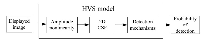
The HVS model addresses three main sensitivity variations. These are the variations as a function of light level, spatial frequency, and signal content. Sensitivity can be thought of as a gain, though the various nonlinearities of the visual system require caution in this analogy. The variations in sensitivity as a function of light level are primarily due to the light adaptive properties of the retina, and we shall refer to this overall effect as the amplitude nonlinearity of the HVS. The variations as a function of spatial frequency are due to the optics of the eye combined with the neural circuitry, and these combined effects are referred to as the CSF. Finally, the variations in sensitivity as a function of signal content are due to the postreceptoral neural circuitry, and these effects are referred to as masking. The HVS model consists of three main components that essentially model each of these sensitivity variations. In the current state of development of the VDP, these three components are sequentially cascaded in the straightforward manner shown in Fig. 1. The first component is the amplitude nonlinearity, implemented as a point process, while the second is the CSF, implemented as a filtering process. The final component in the cascade is the detection process, which models the masking effects. It is implemented as a combination of filters and nonlinearities.
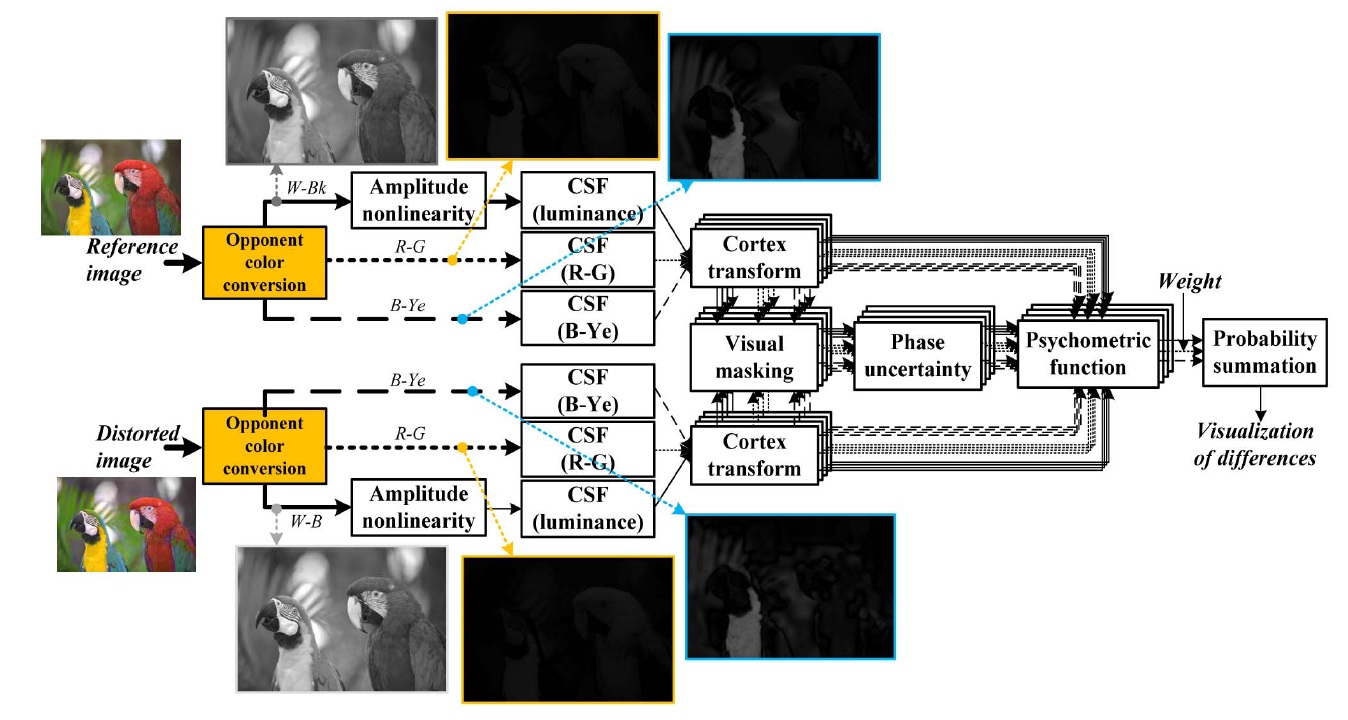
Color components are not as sensitive as luminance components. However, the image quality assessment has to describe the chromatic distortion that cannot be done by a luminance-based system. Thus, we designed an assessment system extended from Daly’s work, as shown in Fig. 2.
For the spatial filtering of opponent channels, white-black (W-Bk), red-green (R-G), and blue-yellow (B-Ye), it is performed using a simple multiplication on a series of convolution. In order to filter the image, the opponent channels must be first transformed into their respective frequency representation using a discrete Fourier transform (DFT). Specifications of the contrast sensitivity functions are used for the general shape of the luminance and chrominance models, as defined by many researchers [6-8]. We use the spatial filters of the S-CIELAB model [9] that are designed to approximate the human contrast sensitivity function for the luminance component as given by:
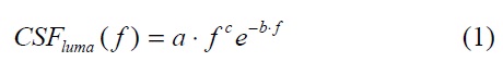
where the parameters a, b, and c are 75, 0.2, and 0.8, respectively.
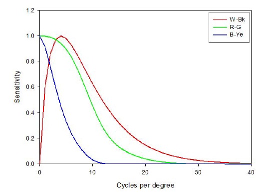
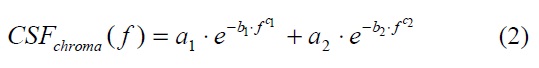
For the chrominance channels, R-G and B-Ye, we use the chrominance CSF filters in Eq. (2), and they are also depicted in Fig. 3. The six parameters are empirically defined.
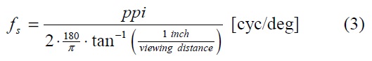
In digital imaging applications, spatial frequency in cycles per degree of the visual angle is a function of both addressability and viewing distance. For example, if a computer monitor is capable of displaying 72 pixels per inch (ppi) and is viewed at 18 inches, then there are roughly 23 digital samples per degree of visual angle. The calculation is shown in Eq. (3) [10]. However, Johnson’s equation should be read in pels/deg instead of cycles/deg.
Since the Poison opponent color space was designed for pattern-color separability, it is useful for implementation of separate contrast sensitivity for each color channel. When applying the CSF to the opponent transformed data, spatial frequencies are calculated by Eq. (3). The luminance data and two color difference data are processed in parallel in the domain of the cortex transform with a reasonable parameter setting.
III. VISUAL ATTENTION MODELING
>
A. Attention Modeling Based on Entropy and Inverse Contrast
It is believed that visual attention is not driven by a specific feature that has dedicated low-level properties that can be treated by the HVS-based assessment. Visual attraction can be induced by either heterogeneous or homogeneous, dark or bright, symmetric or asymmetric objects [11], which is determined by higher level processing than the existing HVS-based system. It can be assumed that image information that is rare in the image, such as high frequency areas or higher contrast areas, will draw more attention. Thus, visual attention may be ascertained by modeling and quantifying the rarity of image information, called entropy [12].
It is well-known that self-information is a function of probability of a symbol. Larger probability gives lower selfinformation by taking a logarithm as
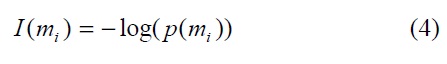
where
A pixel is conspicuous if its gray level is significantly different from the neighboring pixel value. The larger the difference between the two levels, the higher the saliency that it represents. Thus, the saliency value of a level intensity
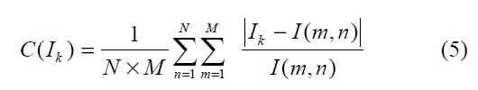
where

The histogram of a digital image with
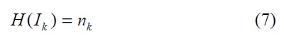
where
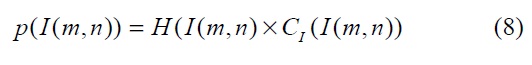
where
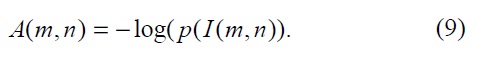
If a message is very different from all the others,
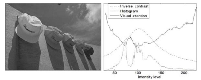
The left and right portions of Fig. 4 show, respectively, the luminance component of the input image and the resulting spatial saliency values, compared with image histogram and global inverse contrast. Note that the scales for three plots are adjusted to represent them on a graph. The lowest saliency is found in the range of frequent occurrences and high global inverse contrast. The saliency values are close to what a human would expect because higher occurrence indicates redundant information in the image, which is, therefore, relatively unattractive (unattended).
The output saliency map shows some important objects obtained by a relatively simple algorithm. However, there may be too many salient objects in the complex images since the map is based on the histogram method. It does not distinguish the semantic meaning of the pixels, size or shape of objects, or texture information. In spite of these limitations, it is still useful for detecting the most salient pixels, which correspond to the pixels of visual attention.
>
B. Attention-based CVDP Modeling
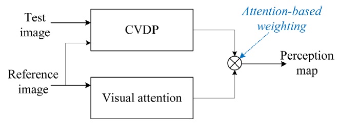
The CVDP utilizes luminance and color responses in HVS and spatial frequency channel sensitivities. However, attention is focused on certain areas of an image that can be modeled by information theory rather than amplitude or frequency responses. Both attention and CVDP systems can be merged in serial or parallel connection. Fig. 5 shows a parallel combination in which visual attention results are weighted to a CVDP map to derive a final visible distortion map.
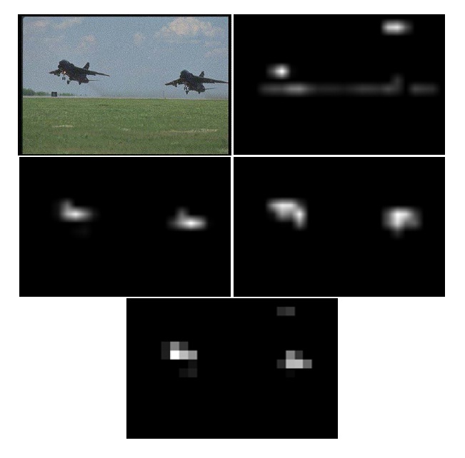
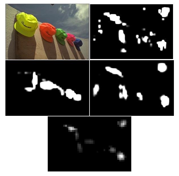
The purpose of visual attention is to determine which objects are the most interesting to the human eye at the moment. However, it is not always object-based. Some regions are most attractive depending on image properties. Itti’s model works well for simple images like Fig. 6, which includes only two aircraft objects. Conspicuity maps for intensity, color, and orientation are separately drawn by considering relevant features. The final saliency map is obtained by combining the three conspicuity maps. However the test image contains only two significant objects, that is, it is so simple. If the complexity of an image increases, Itti’s model does not provide meaningful results as shown in Fig. 7, which contains five cap objects. Although the human eye would be expected to latch on to one or more of the caps that are most attractive, the cap objects are hardly discernible in the final saliency map.
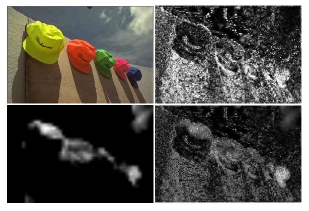
Performance of the proposed attention-based CVDP (ACVDP) scheme is shown in Fig. 8, presenting an original image, CVDP perception map, and attention map obtained by rarity quantified modeling, and the final ACVDP result. It is worth noting that there are some clouds in the top-right part of the distorted “ caps” image that draw quite high attention, but distortions existing inside are not detectable in terms of human sensitivity. On the other hand, the shadow areas below the caps do not draw much attention, but distortions are quite detectable. This means the two different approaches should be closely related to obtain optimum performance.
Image attention models and their application to image quality assessment were discussed. First, the luminance VDP developed by Daly was extended to cover color responses. Color distortions are detected by CVDP. Next, we reviewed the well-organized Itti’s model for image attention modeling. Three parameters, intensity, color, and orientation, are used to generate a saliency map in a hierarchical structure and center-surround technique. Our attention model is based on rarity quantification, which is related to self-information or entropy in information theory. It is based on the fact that more important things are rare. The algorithm is relatively simpler than Itti’s model but results in more consideration of global contrasts from a pixel to a whole image.
The two human eye-related schemes are combined to obtain a more efficient image quality assessment algorithm. The results show that objects that are important in view of one scheme are not really important from the perspective of another scheme. Therefore, the two schemes should be used to compensate for each other.