In this study we investigate the use of 2D and 3D scanning optical coherence tomography (OCT) technology for use in apple blotch diagnosis. In order to test the possible application of OCT as a detection tool for apple trees affected by Marssonina coronaria, we conducted several experiments and compared the results from both healthy and infected leaves. Using OCT, we found several distinctive features in the subsurface boundary regions of both the diseased and healthy leaves. Our results indicate that leaves from diseased trees, while still appearing healthy, can be affected by M. coronaria. The A-scan analysis method confirmed that the boundaries found under the subsurface layers can be faint. This shows that M. coronaria can exert its influence on entire apple trees (as opposed to only on leaves with lesions) once it infects healthy trees. Our results indicate that OCT can be used as a noninvasive tool for the diagnosis of fungal disease in apple trees. Microscopic imaging results, performed as a histological study for comparison, correlated well with the OCT results.
Marssonina blotch caused by
Disease symptoms appear on the leaves and fruits of the affected trees. Although
In order to prevent the transmission of
Recent efforts to compensate for the inadequacies associated with serological and molecular biological methods have revealed challenges regarding the development of new tools for early diagnosis. Efforts have been made to distinguish infected plants from healthy ones by using microscopy and medical techniques, such as X-ray tomography [9], positron emission tomography (PET) [10], magnetic resonance imaging (MRI) [11], and ultrasonography [12]. Most of these approaches are useful in noninvasively capturing morphological and structural plants images, however, they do have limitations. For instance, although a microscope offers a particularly high resolution, there are limitations in its depth scan range and additional preparation needed for histology. MRI and X-ray tomography have low image resolutions that make it difficult to distinguish the microscale features in the samples. PET uses a tracer to enhance its functional imaging, however, the images are not easy to display in real-time. Ultrasonography is a popular imaging modality, however it utilizes an ultrasound gel to increase the transmittances of the ultrasound between tissue and the probe.
Optical coherence tomography (OCT) is a noninvasive optical imaging technique that utilizes a low-coherence interferometer to obtain a high-resolution, cross-sectional image of a biological tissue sample. OCT is an upgraded application of another technique, optical coherence domain reflectometry (OCDR), which was developed in 1987. The first OCT system was developed in 1991 by David Huang at the Massachusetts Institute of Technology [13,14]. The OCT technology has proved to be a useful imaging modality for many biological applications. Owing to its real-time imaging capability and micrometer-scaled resolution, OCT has found important applications in several medical fields, including ophthalmology and dermatology [14-17]. Recently, OCT has found new industrial applications, including the development of security equipment, crack detection, and distinguishing electronic devices [18-20]. Although OCT has a limited scanning depth range (approximately 2 mm) in tissue, it does reveal a greater micro-resolution depth than a microscope. These OCT characteristics are particularly useful to plant researchers, because the OCT scanning depth range is suitable for investigating the inner structure of plant leaves. The use of OCT in plant imaging was first applied approximately 10 years ago in order to investigate the inner structures and morphologies of various plants, including tomatos, kiwifruit, spiderwort, and orach [21-24]. More recently, in 2009, OCT imaging was used to diagnose viral infections in orchid plants and rot in onions [25,26]. Additionally, previous work in our laboratory involved the application of OCT technology to screen virus-infected seeds and to distinguish normal oriental melon seeds [27].
In the current study, we investigated the use of noninvasive 2D and 3D OCT for early diagnosis of the marssonina blotch apple fungal disease. We studied the OCT effectiveness by directly comparing OCT images with microscopic images showing the histology of leaf samples. Computerized A-scan analysis was performed to quantitatively confirm the differences between healthy and infected leaves. Our results suggest that OCT technology can be applied as an early diagnosis method.
The leaves of both diseased and healthy apple trees were collected from the same plantation for our experiments. We prepared samples from similar-sized leaves (4.5 cm × 3 cm) in order to limit any differences arising from the intrinsic growth characteristics of the leaves. We examined the effects of the marssonina blotch caused by
2.2. Optical Coherence Tomography and the A-scan Analysis Algorithm
Healthy and diseased leaves were imaged using a homemade OCT system constructed in our laboratory, which incorporates a super luminescent emitting diode (SLED: 1310 nm central wavelength, DensLight) with a 3 dB band
width covering 150 nm. The sample arm has an objective lens (Thorlabs LSM02, NA = 0.37, f = 1.8 mm) and 2 galvo-scanners that image using C-mode scanning. Our scanning range was 2 mm × 2 mm. This OCT system produces a micro-resolution image with an axial and a lateral resolution of 6.7 μ m and 17.3 μ m in the air, respectively. The numbers of A-scans needed to obtain the 2D and 3D images were 200 and 512, respectively.
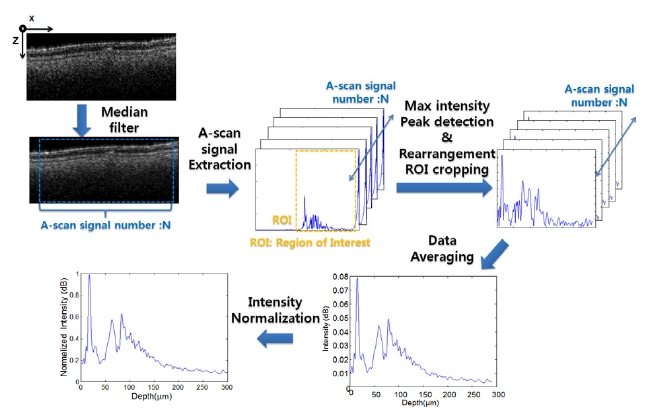
A-scan analyses were performed in order to more clearly observe the differences among the layers of the samples at a micro scale level. For use in conducting the automatic clarification of the layers, an A-scan algorithm was developed using MatLAB (Mathworks 2009). The data analyzed were obtained from the saved 3D volume images. The schematic diagram shown in Figure 1 illustrates the mechanism used to acquire the layer information. X-axis and z-axis in figure 1 are OCT B-scan direction and A-scan direction, respectively. First, the demodulated raw data were processed, and then the selected image was cut from the cross-sectional 2D images. A median filter was also applied to compensate for the speckle noise in the A-scan signals, which can result in erroneous peak detections. N numbers of A-scan signals were extracted from the filtered image. From the coded program, the first peak was determined by finding the maximum value intensity peak among the unpredictable value intensity peaks in the depth axis direction. The processed data set was then rearranged to establish the first peaks. After cropping the region of interest (ROI), the processed A-scan signal data were averaged. In order to acquire a stable intensity profile, the A-scan signal intensities were normalized by dividing them into the max value. From the acquired A-scan profile, we were able to analyze the various conditions of the layers, such as the number of peaks.
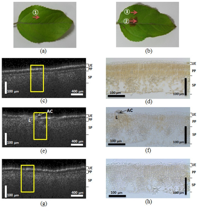
As shown in Figure 2, the OCT images of non-symptomatic
leaves from a healthy tree and lesioned and unlesioned segments on an abnormal leaf from a diseased tree were compared. The appearance of the structures imaged by the OCT corresponded well to the histological images obtained from optical microscopy. The yellow boxes in Figure 2 indicate corresponding areas in the microscopic images. Figure 2 (a) shows a photograph of the normal leaf from the healthy tree. The arrow ① indicates the transversal scanning direction over the 2 mm scanning range. We found that the OCT images closely corresponded to the microscopic images. The OCT image from Figure 2 (c), which shows the normal leaf (Figure 2 (a)), showed distinctive boundaries between the 3 layers of the leaf (upper epidermis (UE), palisade parenchyma (PP), and spongy parenchyma (SP)). Figure 2 (d) shows the corresponding microscopic image of the normal leaf structure, which also reveals the three distinct layers. However, due to the shrinking that occurred during the preparation of the histological slides, the boundary gap between the UE and PP layers was smaller than that observed in the OCT images (Figure 2 (c)). Figure 2 (e) is the OCT image of the lesions on the abnormal leaf. We acquired the image by scanning in a transverse direction, as indicated by arrow ② in Figure 2 (b). This image also reveals broken layers between the PP and SP layers, and under the UE. The microscopic image in Figure 2 (f) also exhibited unclear, indistinct layers. This is especially apparent on the left side of the the fungus acervuli (Character AC) in the microscopic image, which shows broken UE layers that were also detected on the left side of the yellow box from Figure 2 (e). These results suggest that the OCT can be successfully used to diagnosis the differences between normal leaves in a healthy tree and abnormal, infected leaves from diseased trees.
In order to explore the distinctive difference between the normal and infected areas of the infected leaves, we also imaged a normal area approximately 6 mm away from where the lesion image was acquired, as depicted in Figure 2 (g). Arrow ③ in Figure 2 (b) represents the transverse scanning direction of the normal area. When we compared this image to the Figure 2 (c) image, the second layer between the PP and SP layers was unclear. The microscopic image shown in Figure 2 (h) also reveals a similar symptom, where the boundary between the PP and SP layers is difficult to distinguish. This second experiment revealed that the normal area in the infected leaf, which had all the appearances of being a normal leaf, also contained changes in the inner tissue structure that were present in the lesion areas caused by the fungi.
3.2. 3D OCT Imaging in the Infected Leaf
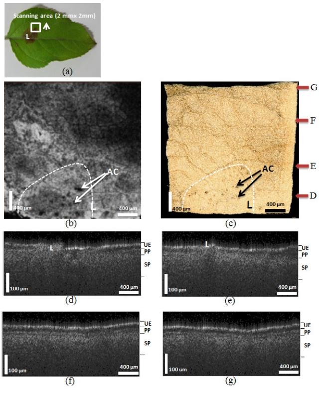
In order to reveal the effect of the fungus on the lesion area margin, we performed 3D scanning (2 mm × 2 mm) on selected areas (Figure 3 (a), white box) containing the margin of the lesion. The sample used in this particular experiment (Figure 3 (a)) was the same leaf used in the first experiment. The arrow in Figure 3 indicates the area measured and the scanning movement direction. Figure 3 (b) shows an enface leaf image revealing that the lesion (white dotted line) area, which looks like a dark brown spot, contains the fungus acervuli (Character AC).
Figure 3 (c) shows the 3D scanning area images. The red arrows represent the cropping point used to show the cross-sectional images in Figures 3 (d)-3 (g). Figures 3 (d)-3 (g) show the OCT images acquired after scanning the indicated areas along the arrow. Figure 3 (d) includes the OCT image of the lesion itself. After comparing these OCT images, we concluded that the UE, PP, and SP layers were increasingly more distinctive. This result confirms that the fungus spread outward from the lesion. Figures 3 (f) and 3 (g) appeared similar to Figure 2 (g). Therefore, we also concluded that the fungus migrated up to arrow F (approximately 1.5 mm) in the scanned area.
3.3. The Normal Leaf Comparison between the Healthy and the Diseased Tree
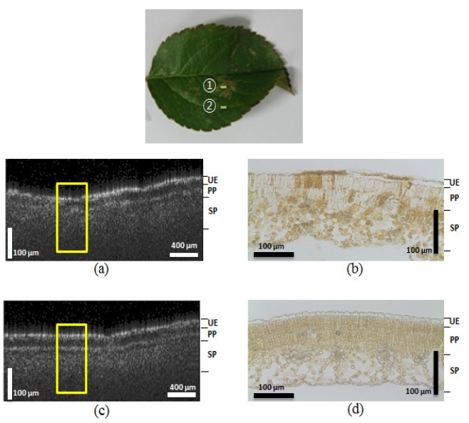
In order to reveal more detailed information about the influence of the fungus on normal leaves obtained from what appears to be a healthy tree, we used both the 3D
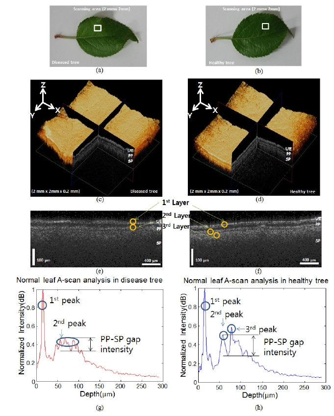
OCT imaging and the A-scan analysis method to compare the normal leaf samples from both healthy and diseased trees. Figures 4 (a) and 4 (b) show the normal leaves from the diseased and healthy trees, respectively. The white boxes in Figures 4 (a) and 4 (b) define the scanning area (2 mm × 2 mm). Figures 4 (c) and 4 (d) show the 3D OCT volume images of the diseased and healthy trees, respectively. Figures 4 (e) and 4 (f) show the cross-sectional OCT images of the diseased tree and healthy tree, respectively, acquired by scanning areas in similar positions on each of the leaves. After analyzing the OCT images of the 2 normal leaves, we noticed that it was more difficult to identify the boundaries among the layers under the UE in the diseased leaf compared to that found in the healthy leaf. We also utilized the A-scan analysis method to assess these leaves. For the A-scan analysis, the first peaks in the depth direction were searched for in the OCT B-mode, which was later rearranged to flatten the first peaks. The A-scans were sampled and averaged from the flattened first-peak B-mode image. Figures 4 (g)-4 (h) show the results
of the normalized A-scan analysis. The X-axis and Y-axis represent the depth length and the normalized intensity (dB) of the OCT signal, respectively. The first peak, which is representative of the UE layer, was found to be the same in Figures 4 (g)-4 (h). However, the other peaks were different for the different leaves. Figure 4 (g) does not show the third peak clearly; the second peak has a broader profile than that found in Figure 4 (h). This result gives detailed information about the broken boundary between the PP and SP, and is consistent with the OCT images shown in Figures 4 (g)-4 (h). A small decrease in the intensity in the OCT signal presents itself in the middle of the second peak, as shown in Figure 4 (g). However, this decrease is larger in the healthy sample (Figure 4 (h)) compared to that found in the seemingly healthy one (Figure 4 (g)). We measured the condition of the leaf quantitatively by defining the PP-SP gap intensity as the difference from the
PP peak to the lowest intensity value between the PP and SP. The PP-SP gap intensity between the diseased and the healthy tree were measured as 0.132 dB and 0.308 dB, respectively. When we conducted the same calculation with 10 other samples, the PP-SP gap values in the two cases were statistically different: 0.108 ± 0.043 dB and 0.298 ± 0.075 dB, respectively.
3.4. The Diseased Leaf Comparison between the Wormeaten and the Fungus Infected Leaves
We compared the OCT imaging results revealing the fungus-induced changes in the leaves to the results of a worm-eaten leaf that was attacked by Pear lace bugs. The morphological destructive pattern in the worm-eaten leaf was expected to be different from that found for the fungus-induced leaf. The lesion shown in the top panel of Figure 5 is similar to the fungus-induced lesion on the abnormal leaf, shown in Figure 3. Labels ① and ② indicate the traverse scanning directions on the lesion and the normal area, which was 6 mm away from ①. It was difficult to visually assess with the naked eye which leaf was indeed the worm-eaten leaf. The OCT image of the lesion on the worm-eaten leaf was almost identical to that of the infected, abnormal leaf shown in Figure 3. However, when we scanned the area of the worm-eaten leaf 6 mm away from the lesion, the OCT imaging revealed clear boundaries for the layers. We saw broken layers only in the wormed lesion area.
We have investigated the possibility of using OCT technology for the diagnosis of marssonina blotch through the analysis of data from several different experiments. Through the OCT scanning experiments we learned that if a leaf has been influenced by the fungus the structure and distinction of its layers became somewhat unclear in the OCT images. This is probably because the fungus penetrates the inner apple leaf during infection, destroying many cell components in the leaf, including the UE, PP, and SP. Each component of the leaf tissue has a unique refractive index. The differences in these refractive indices play an important role in the scattering from the boundaries of the components. The OCT interference signals are derived from the scattering found at the boundaries of the tissue layers. Therefore, if the components of the layers are destroyed by certain factors, such as fungi, viruses, or germs, they lose their unique refractive index. If the difference in the refractive index is not distinct, the scattering signal will be inadequate. When an OCT beam is focused on a healthy tissue, a highly sensitive scattering signal is detected that represents the normal distinctive OCT layers. However, if the layers are partly destroyed, the scattering at the boundary will be particularly weak, thus generating a profile obviously different than that found for a sample with readily discernible layers.
Our first experiment (Figure 2) confirmed that OCT technology can be used to distinguish between the lesioned areas of infected leaves compared to healthy leaves. Specifically, the OCT imaging revealed the broken layer structure in areas with surface lesions. In addition, we observed that a seemingly normal area of an infected leaf may include broken layers. This finding indicates that the OCT can reveal not only lesions but also infected areas that are impossible to distinguish with the naked eye. Our second experiment (Figure 3) provided additional information about the infection process and its impact. Specifically, we determined that even though a leaf area may appear normal, its layers may already be destroyed by the fungus. By transverse scanning of a leaf at regular intervals along a region close to a lesion (2 mm × 2 mm), we were able to infer the extent of the fungal activity in the infected leaf. We found that the actual infected area to 1 side of the lesion was 1.5 mm, when measured from the center of the lesion. The actual entire infected range could also be measured simply by scanning the entire area around the lesion. Our third experiment (Figure 4) confirmed that a normal-looking leaf from a diseased tree, although seemingly healthy, might still be affected by the fungus as revealed by loss of the boundary distinction between the PP and SP layers. Furthermore, the A-scan analysis method confirmed our OCT experiment results. This shows that the fungus can exert its influence on an entire apple tree (as opposed to leaves with lesions only) once it infects a healthy tree. Our fourth experiment (Figure 5) showed that the OCT can distinguish between leaves affected by the fungus and those that are abnormal for other reasons. Specifically, we scanned a worm-eaten apple leaf and compared it to leaves having the fungal infection. We found that in the fungus infected leaves, the lesion as well as the surrounding area was affected, whereas, in the worm-eaten leaf only the lesioned area was affected.
All of our experiment results can be explained by an inherent plant defense mechanism. Generally, plants infected with a pathogenic bacterium/fungus produce a self-defense response due to systemic signals [28]. Previous studies have reported upon the morphological self-defense mechanisms of plants, such as the accumulation of hydroxyproline-rich glycoproteins (HRGP) in plant cell walls and the lignification of the cell walls. These defense responses appear to impede the growth of the pathogenic bacterium/fungus in a host and directly protect it from secondary invasions [29]. In the case of a melon inoculated by an anthracnose, the continuity of the HRGP response generation in the cell has been confirmed [30]. These reports strongly suggest that if the host is infected by a pathogenic bacterium/fungus, changes will be observed in other tissues radiating outward from the tissue where the infection occurred as a result of a systemic signal. Therefore, the above evidence indicates that OCT technology can be used to diagnosis fungal infections in apple trees. There are other fungal diseases that can infect apples, such as bitter rot and white rot on the fruit, and rust and alternaria blotch on the leaves. Rust and alternaria blotch are minor and show disease symptoms, such as spots that can be seen by the naked eye, within 2~3 days after infection. In the case of Marssonina blotch, the visible symptoms can only be seen after at least 2~3 weeks after infection or 4-5 weeks if the latency period is long [31]. Due to the long latent period of this disease, early detection using the OCT method would be very helpful for protection against this disease with suitable control program, such as fungicide spraying.
Our results demonstrate that OCT technology can be used to distinguish the inner cross-sectional layers of a lesion in a diseased leaf from the layers of a healthy leaf. We also demonstrated that this method can reveal the specific infected area of an abnormal leaf, as well as the strength and direction of the activity of the fungi. This information is useful to farmers who wish to take preventive measures against fungal diseases affecting apple trees. Based on these results, we conclude that OCT technology can be used as an early diagnosis tool, because it able to reveal the distinctive characteristics of a seemingly normal but actually infected leaf from a diseased tree. A practical diagnosis can be conducted in the field test by utilizing a handheld probe and a next stage portable and high speed OCT system [32]. The upgraded OCT system and accessories are expected to increase the reliability of our research and afford an opportunity to extend this application to other crops.