Low-crosstalk arrayed waveguide gratings (AWGs) are key components in dense wavelength-division-multiplexing (DWDM) photonic networks [1]. The crosstalk depends on the phase errors of the waveguide array and can be reduced by various compensation techniques requiring precise phase measurements [2-4].

The phases of an AWG can be measured by an optical low coherence method [5-7] or by a frequency domain method [8-10]. The latter method is easier to implement because it does not require fine control over the path length in an interferometer. In this method, the phases are obtained from the Fourier transform of the interference intensities, which appear as a series of peaks that have the phase information of each waveguide. However, it is impossible to completely eliminate overlaps of neighboring peaks. Hence, another process is required to extract the phase values. The measurement accuracy may also be lowered by the error in calculating the Fourier transform.

In this paper, we propose a method to obtain phase values directly from the interference intensities, without the need for Fourier transformation. We verify this approach by a simulation in which an artificial AWG is analyzed. In section 2, we describe the method of phase measurement. The results of the simulation are reported in section 3.

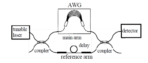
Figure 1 shows a schematic diagram of the experimental setup for the frequency domain method. The AWG is included in an arm of a fiber interferometer, and the interference intensity is measured as a function of the laser frequency.

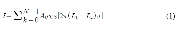
When the AWG is composed of N-waveguides, the interferogram, which is defined as the normalized AC component of the interference intensity, can be expressed as follows [11]:

Here, A_k is the amplitude of the transmittance of the k-th waveguide, L_k is the length of the path containing the k-th waveguide including the effect of the refractive index, L_r is the path length of the reference arm, and σ is the

reciprocal of the laser wavelength. L_k can be expressed as L_k=L_o+kΔL+_？k, where L_o is the length of the path containing the shortest waveguide (k = 0), ΔL is the step increment, and _？k is the error in the step increment.

We derive the values of the amplitudes and lengths by fitting the theoretical interferogram to the experimental data through the Monte-Carlo method. The process is as follows. First, we assign initial values to the set of parameters {A_k, L_k}. Either uniform, Gaussian or sinc distributions can be assigned initially to {A_k}. The initial values of {L_k} may be given randomly, however the computational time can be reduced by starting with the ideal lengths of the AWG. Using the initial values, we calculate the cost function, which is defined as the sum of the squared differences between the theoretical and the experimental interferograms over σ. Next, one of the parameters is chosen randomly and changed slightly. If the cost function increases, the value of the changed parameter is restored. If the cost function decreases, the change is accepted. This process is repeated until the cost function converges. We wrote a program for the process of automatic optimization. The last set {A_k, L_k} includes the desired amplitudes and phases.

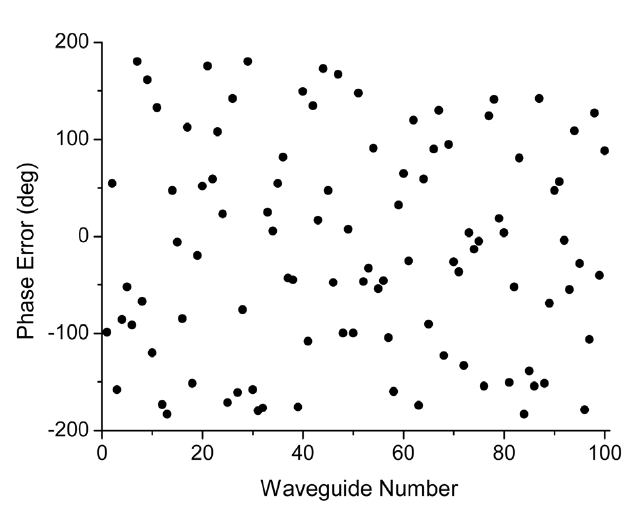
We simulated the phase measurement process to verify our method. First, we created an artificial AWG with arbitrary phases and amplitudes. Then, we calculated the virtual interferogram by using Eq. (1). Considering this as an experimental interferogram, we derived the phases and compared them with the initially given values.

The number of waveguides in the array (N) was assumed to be 100. A random length error (_？k) within a wavelength was given initially to each waveguide. Figure 2 shows the given errors, which were converted to the phase values for the central wavelength. The amplitudes were given as either Gaussian, sinc or uniform distribution. The laser wavelength of the interferometer was assumed to be scanned from 1500 nm to 1600 nm. Then, the value of Δ_σ was equal to 0.042 μm^-1). The path difference L_o- L_r was fixed at 10 mm

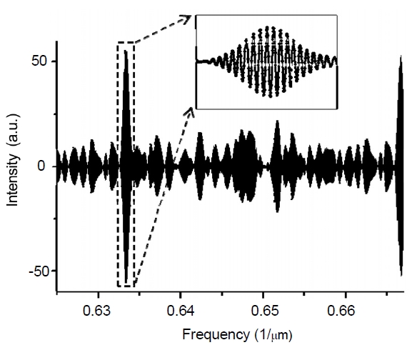
Figure 3 shows an example of a virtual interferogram for an AWG whose step increment (ΔL) is equal to 50 μm.

The symbols in the inset represent the theoretical data fitted by the Monte-Carlo method. Here, 10000 data points for σ are used to calculate the cost function. The computer running time for the Monte-Carlo-optimization is approximately 5 minute. We can see in the figure that the intensity oscillates with σ. The period depends on the value of L_o-L_r. The interval between the two peaks corresponds to the free spectral range (FSR), i.e., the reciprocal of ΔL.

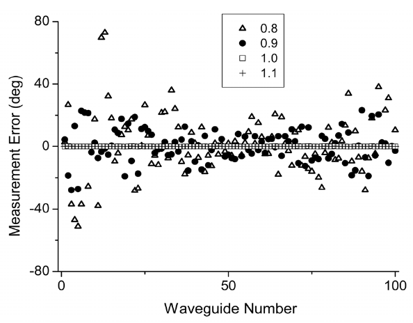
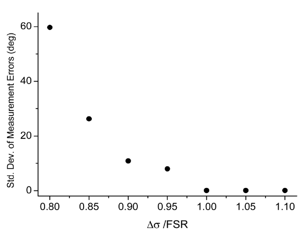
Previous studies have shown that the possibility of phase measurement depends on the laser tuning range (ΔL) of the interferometer. Hence, we measured the phases for various ratios of the tuning range to FSR (Δσ/FSR). The results are shown in Fig. 4. The vertical axis represents the phase measurement error, which is the difference between measured and the given lengths of each waveguide. The numbers in the box indicate the values of Δσ/FSR. As we can see in the figure, the measurement errors are nearly zero for all the waveguides if the ratio is equal to or

greater than 1.0. However, as the ratio becomes less than 1.0, the errors increase rapidly. Figure 5 shows the standard deviation of the phase errors. The deviation is 0.07° when the ratio is 1.0. However, it increases to 8° when the ratio is 0.95. Hence, we can conclude that the phases can be measured correctly if Δσ is greater than the FSR.

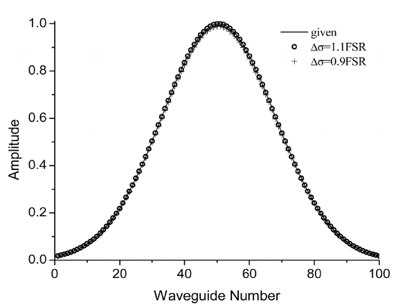
The relative amplitudes were also measured for various ratios Δσ/FSR. Figure 6 shows the measured amplitudes when Gaussian distribution was given to an AWG. The measured amplitudes are in good agreement with the given amplitudes even when Δσ is less than the FSR. We got the similar results even if we start the Monte-Carlo process with other initial amplitude distribution. When a sinc or uniform distribution was given to the amplitudes, the measurement errors were also negligible regardless of the initial conditions. Hence, we can conclude that amplitude measurement is insensitive to the experimental condition.

When we used a trial-and-error method in Fourier space, we could measure the phases precisely only if Δσ was larger than 1.7FSR and the phase errors were given within

50° [11]. And even in that case, the measurement errors were very large for waveguides with amplitudes lower than 20 % of the peak value. The standard deviation of the phase measurement errors was greater than 1°, which is more than ten times of that in intensity space. Above all things, computational time of the Monte-Carlo process is much longer in Fourier space than in intensity space. Hence, it would be more advantageous to measure them in the intensity space. The poor results in Fourier space are believed to be related to the errors in calculating the Fourier transform.

We show that it is possible to measure the phases of an AWG directly from the interferogram by a trial-and-error method. The phase measurement error is as low as 0.1° if the laser tuning range is greater than FSR. Moreover, this method shows high performance even for waveguides at the edges of the array, which tend to have very small amplitudes. All the characteristics are superior to the analysis using the Fourier transform.