It is very important to analyze effectively the tolerance of an optical system with high resolution as the projection lens of photolithography or as the objective lens of a microscope. We would like to find an effective assembly structure and compensators to correct aberrations through global wavefront sensitivity analysis using Zernike polynomial expansion from the field and pupil coordinates rather than from only pupil coordinates. In this paper, we introduce global wavefront coefficients by small perturbations of the optical system, and analyze the optical performance with these coefficients. From this analysis, it is possible to see how we can enlarge the tolerance through the proper assembly structure and compensators.
In general, the tolerance analysis of an optical system has been regarded as one of the analysis processes to get allowable errors in manufacturing and assembly and many studies to get the tolerance also have been conducted [1-10]. As the needs with regard to optical system performance are increasing, however, tolerance analysis needs to be understood as a process to maximize the tolerance rather than merely as a process to acquire the tolerance for production. To this end, the fundamental element is to design the optical system with loose tolerance. In general, however, the tolerance of an optical system with a large Numerical Aperture (NA) should be tight indeed. In consideration of this limitation, a way of maximizing the tolerance is to analyze the effect on optical aberrations in detail caused by the errors in manufacturing and assembly of each element of the optical system (hereunder, these errors will be called optical perturbations), and to find the optimal assembly structure and compensators with which the tolerance could be maximized. Some of the commonly used compensators include image focus, image surface tilt, z axis moving of a lens, and tilt or decenter in direction of the x and y axis of a lens. The problem is, how could we find such compensators, and how could we find the assembly structure to maximize tolerance? Mostly, such factors as modulation transfer function (MTF), root mean square (RMS) wavefront error, or Strehl ratio may be adopted as the criteria for optical performance. They may indicate the performance of an optical system as a single value, but it is not evident how each element error of the optical system specifically affects the optical system performance [8-10]. In other words, only based on these single values, we cannot know what kind of aberration will appear by optical perturbation. Also it is very difficult to find the phase of aberration in relation to the relative changes among errors. One of the ways to solve this problem is to analyze the wavefront deformation regarding optical perturbations and it may be sensitivity or reverse-sensitivity analysis using Zernike polynomials for each field [11]. It is useful to analyze the optical system with a small field [12]. This type of analysis, however, should involve the individual analysis for each field and integrate them. It is very bothersome to consider the optical system condition over the entire field. In particular, it is not easy to analyze the tolerance for distortion with these wavefront deformations depending on the fields separately.
As the wavefront deformation of a certain field cannot represent the general characteristics of the optical system, there is limitation when the optical system performance is analyzed with a certain field merely by means of conventional wavefront representation in Zernike polynomial expansion from the pupil coordinate. In this context, this wavefront aberration in each field may be spoken of as zonal wavefront aberration.
In contrast, the wavefront aberration representation in Zernike polynomial expansion from the both of pupil and field coordinates will be called the global wavefront aberration [13, 14].
Note that this global wavefront aberration is the wavefront deformation due to small optical perturbation with representation in Zernike polynomial expansion from the pupil and field coordinate.
In this paper, we introduce the general global wavefront aberration and get the global wavefront coefficients with an unobscured optical system. And then we will find out how to get the optimal compensators to maximize the tolerance and the optimum assembling structure to keep the best optical performance based on the analysis of such global wavefront coefficients.
II. GLOBAL WAVEFRONT ABERRATION
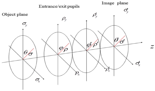
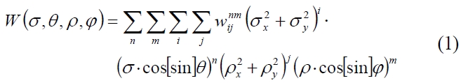
Hereafter, the normalized field and pupil coordinates are introduced as Fig. 1 in order to mathematically express the global wavefront deformation by an optical perturbation in utilization of Zernike polynomial expansion
where (
The chief function determining all the aberration properties is the global wavefront deformation being the function of four monochrome variables,
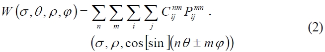
The alternate expansion of the function W can be obtained through the orthogonal Zernike polynomial series as Eq. (2) [13, 14].
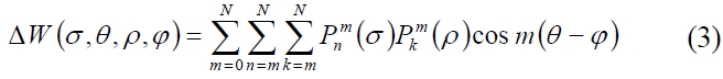
For centered systems, the global wavefront deformation by symmetric small optical perturbation (radius, thickness etc) will look like Eq. (3) [14].
where
For any optical system, the global wavefront deformation by non-symmetric small optical perturbation (lens tilt, lens decenter, surface tilt, surface decenter etc) can be expressed as Eq. (4) [14].
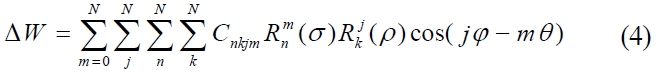
where j = m ± s and s = 1, 2, 3...
In general, for any optical system with symmetric or non symmetric optical perturbation, the global wavefront deformation can be expressed as Eq. (5) from Eq. (3), Eq. (4) and integers,
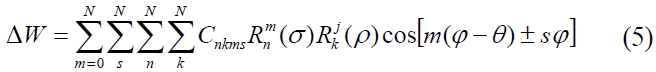
where m = j (s = 0) indicates the centered perturbation, and m= j ± 1 (s=1) for the decentered perturbation due to such factors as small tilt and decenter. In the case of small perturbation, s=1 would be enough. As the amount of perturbation increases, the high order s should be taken into consideration.
One aspect to be noted here is that the global wavefront coefficients
The meaning of the coefficients
1) For centered optical perturbation system (s = 0)
C020=DW0/020 : Defocus
C220=DW0/220 : Field Curvature
C040=DW0/040 : Spherical Aberration
C111=DW0/111 : Magnification error
C131=DW0/131 : Coma
C222=DW0/222 : Astigmatism
C311=DW0/311 : Centered Distortion
2) For decentered optical perturbation system (s = 1)
C120+=DW1/120+ : Field Curvature with dependence of field and azimuth angle
C011-=DW1/011- : Image shift
C031-=DW1/031- : Constant Coma
C122-=DW1/122- : Astigmatism with linear field dependence
C211-=DW1/211- : Cylindrical Distortion (1st Quadratic distortion)
C211+=DW1/211+ : Perspective Distortion (2nd Quadratic distortion)
C231-=DW1/231- : Coma with dependence of field and azimuth angle
C231+=DW1/231+ : Coma with dependence of field and azimuth angle
C233-=DW1/233- : Astigmatism with dependence of field and azimuth angle
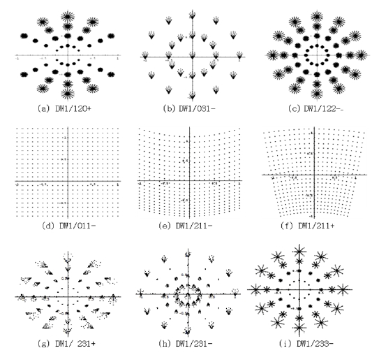
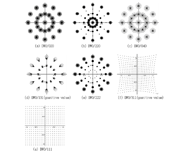
where the last index + and - means +1 and -1 respectively. i.e. C2111=C211+ and C211-1=C211-. Also instead of C notation we use DWs/nkm±s. It is easy to understand the meaning of each coefficient through the spot diagrams in the image plane as Fig. 2 and Fig. 3.
Now we can get all information of aberrations for optical small perturbation. If we can analyze the relations of these aberrations with size and direction between these optical perturbations, we can have a good solution to enlarge the
tolerance of an optical system with the global wavefront coefficients. Also, if an aberration by an optical perturbation has a high sensitivity and other aberrations are small, then we can use this element as a compensator to compensate the aberration with the high sensitivity.
Let’s find optimum compensators and best assembling structure to enlarge the optical tolerance using global wavefront coefficients in Eq. (5) which indicates the global wavefront deformation due to the centered and decentered small optical perturbation. In this paper, we use the exposure optical system with the two important indexes of performance, resolution and distortion, for the analysis with these coefficients.
Let’s choose the projection lens with line and space 3 μm, maximum distortion 0.5 μm, magnification -1, wavelength 405 ± 2.5 nm and field half size 20 mm.
It is reasonable to choose NA = 0.1 of projection lens through the analysis of contrast with 3 μm square line pairs. We can see the contrast has 0.76 with incoherent light source using ideal lens with NA = 0.1. In general, it is acceptable for the contrast to have more than 0.6 for projection lens of photolithography, so we have enough manufacturing tolerance more than 20% in resolution.
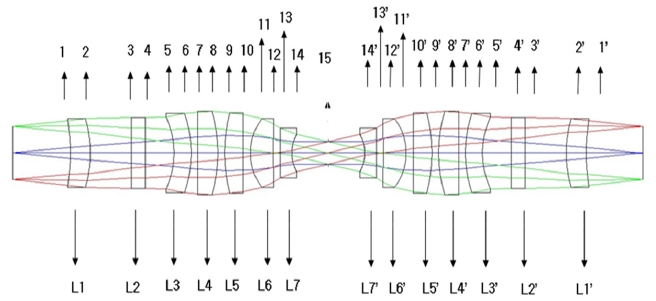
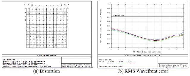
We will analyze wavefront sensitivity with the optical system as shown in Table 1 which has the symmetrical structure with the stop at the center (the layout is Fig. 4). This type of optical system features that the value of the coma, distortion and lateral color are all zero. However, these aberrations appear by the fabrication and assembling errors of optical system, and thus it is necessary to thoroughly analyze for all aberrations.
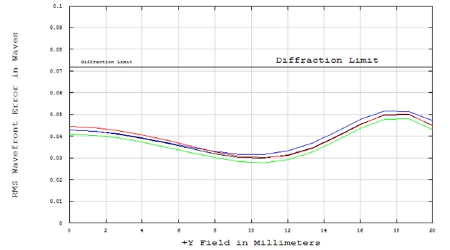
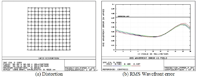
The RMS wavefront error of the current optical system is as Fig. 5:
Let’s analyze the sensitivity of the global wavefront aberr-
[TABLE 1.] Lens data for tolerance analysis
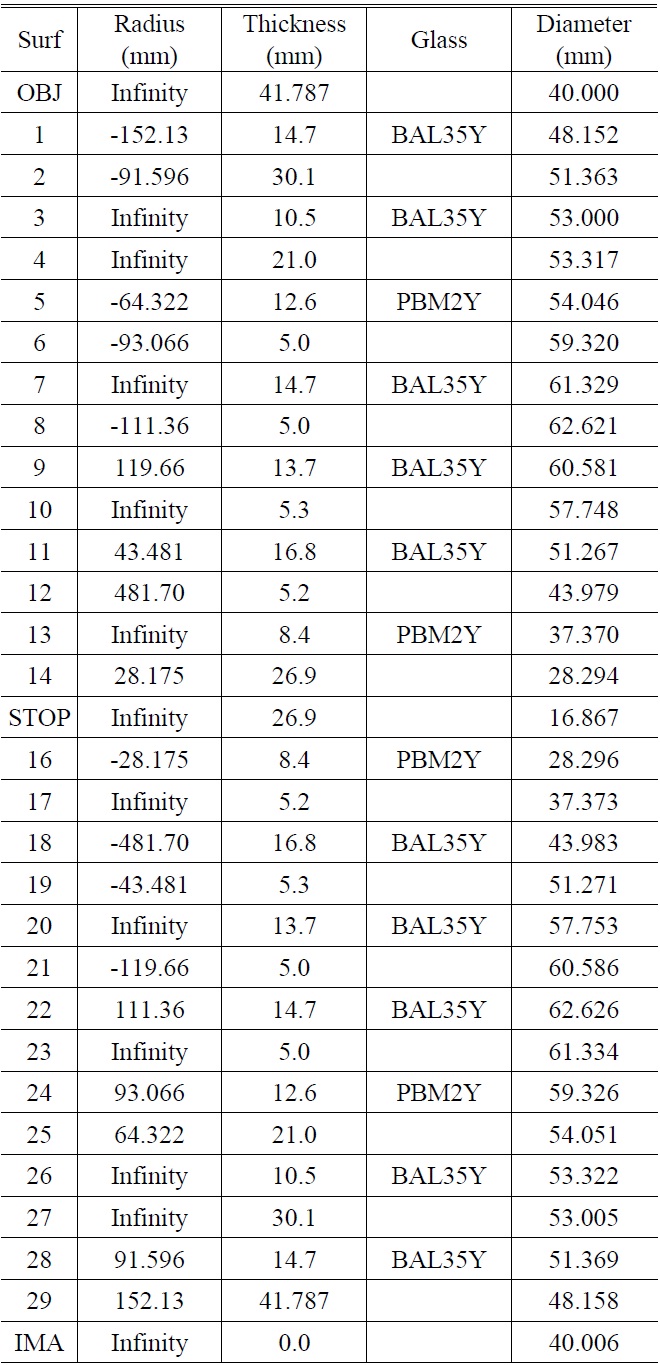
Lens data for tolerance analysis
ation by perturbed optical system. The global wavefront coefficient can be drawn under the condition that minimizes the error function in Eq. (6) [16].

where ΔW=Wori -Wper indicates the wavefront deformation due to a small optical perturbation, F is Zernike polynomial expansion from the field and pupil coordinates as in Eq. (7).
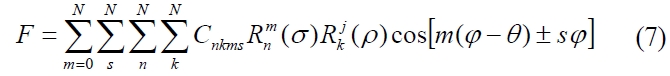
In this paper, it is considered just in case of s=0 and 1, because s=0 and 1 would be enough for a small optical perturbation in considering tolerance. Eq. (7) is the case for decentering over axis y (tilting over axis x) as perturbation. For decentering over axis X (tilting over axis y), we will have sin[m(
3.1. Lens Decenter as Perturbation
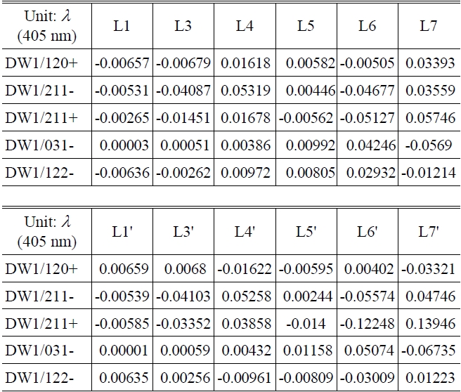
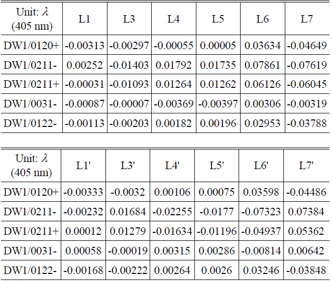
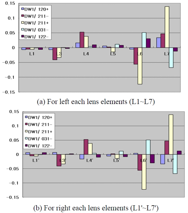
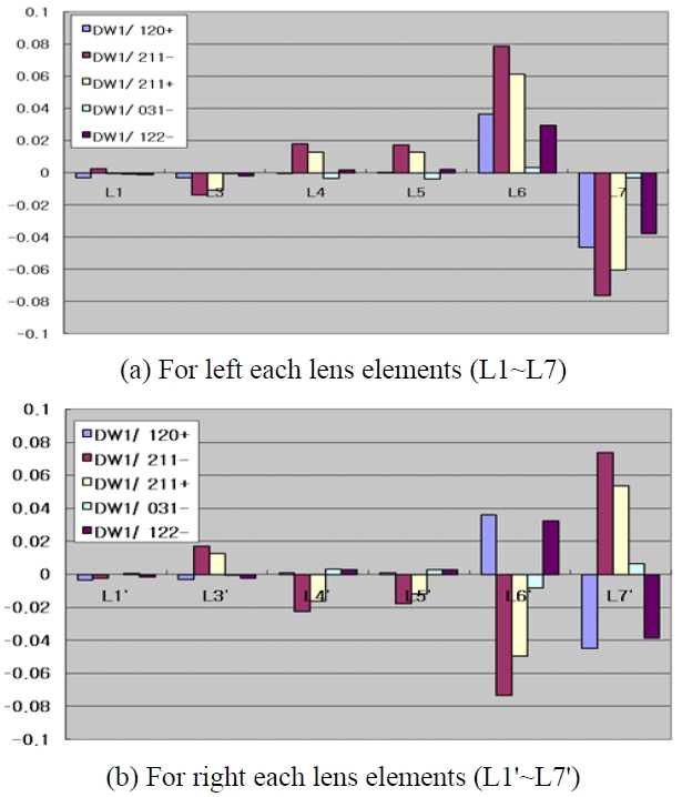
Let’s consider the case of the wavefront deformation due to lens decenter over y axis in the assembly process. As each lens element is decentered as much as 50 μm in the optical system in Table 1, the global wavefront coefficients from Eq. (6), Eq. (7) and s=1 are as in Table 2, where we consider just five coefficients because the others are so small. Table 2 can be expressed schematically as Fig. 6.
Figure 6 indicates the following aspects. First, it shows that L6 and L7 are of high sensitivity. However, the sign of coefficients related to each decenter of L6 and L7 are contrary to each other, and the sizes between them are very similar except for DW1/120+. The fact above indicates that most of the aberrations are removed except DW1/120+ when L6 and L7 are decentered in the same direction. In addition, it shows that DW1/120+ for L6 and L7 are relatively small and in the direction of counterbalance. Thus, if L6 and L7 go through a precision assembly and then assembly to the lens barrel as a group, the aberrations
[TABLE 2.] Global wavefront coefficients by 50 μm decenter of each lens element

Global wavefront coefficients by 50 μm decenter of each lens element
due to the group decenter error of L6 and L7 would be much less effective. Besides, The decenter of L6 and L7 may be used as the compensator to compensate for the Field Curvature of the type of DW1/120+. L6' and L7' to show the same results with L6 and L7.
Second, It shows that as to L3 and L3', other aberrations than the cylindrical and perspective distortion were quite insignificant. Thus, L3 and L3' are very appropriate as the
compensator to correct the distortion. In conclusion, if L6 and L7 & L6' and L7' are assembled as a group respectively, it would be advantageous in keeping the performance of the optical system, and L3 and L3' could be adopted as the compensator to correct the distortion. The validity of the analysis above is verified as direct analysis with optical design S/W.
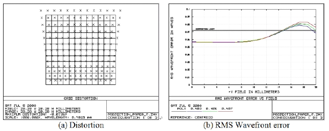
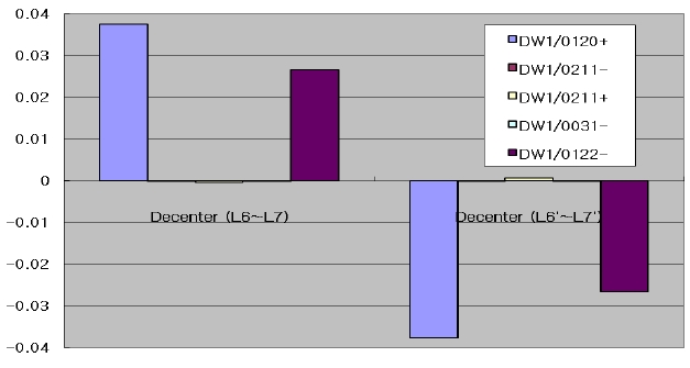
Figures 7 and 8 show the RMS wavefront error and distortion when L6 and L7 lenses are decentered 50
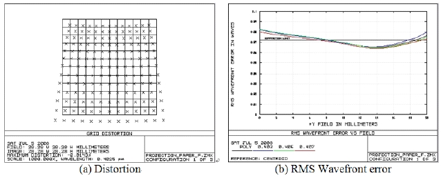
Figure 10 shows the result of decentering L3 lens as much as 100 μm. When the distortion changed as much as 0.013%, the value of RMS wavefront changed very little.
[TABLE 3.] Global wavefront coefficients by tilt(one arcmin) of each lens element

Global wavefront coefficients by tilt(one arcmin) of each lens element
Thus, it is verified that the use of L3 Lens decenter might compensate for the distortion.
3.2. Lens Tilt as Perturbation
The wavefront deformations due to lens tilt indicated in this assembly with the lens decenter are analyzed hereunder.
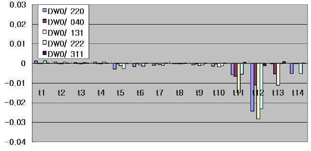
In the optical system shown in Table 1, the global wavefront coefficients to the lens element tilt of one arcmin are as Table 3 and as Fig. 11 schematically.
Figure 11 shows that every aberration had opposite sign to each other for lens tilt of L6 and L7 as in the decenter of the lens. In particular, as all included the field curvature, unlike the case of lens decenter, the absolute values of all aberrations are similar to one another. It turned out that mounting of L6 and L7 as a group in reflection of the characteristics of decenter and tilt of L6 and L7 is quite advantageous in achieving the goals in relation to the performance and distortion of an optical system. The demonstration of the factors above could be verified by means of such factors as lens decenter.
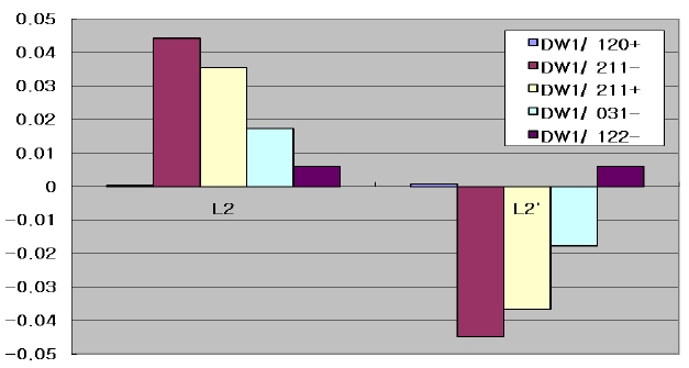
Let’s examine the wavefront deformation in reflection of the plate tilt of L2 and L2'.
Figure 12 shows that all coefficients except DW1/122-
had the opposite sign, which indicates that when plates L2 and L2’ are tilted to the same extent in the same direction, all aberrations except astigmatism are offset. In particular, although this is a natural result, the distortion is completely offset and becomes zero. In short, the tilt of plates L2 and L2’ could be used to compensate for astigmatism.
As to the relative decenter(50 μm) of the left side (L1~L7) and right side(L1'~L7'), the result is presented in Figure 13, which indicates that the half decentering of the optical system might change the field curvature and astigmatism with no effect on the distortion. It might be compensate field curvature and astigmatism with this decenter.
This analysis above, in addition to analyses on methods to minimize aberrations and compensators, shows the extent of sensitivity depending on the manufacturing and assembly errors of an optical system. Axis y of each Figure shows the changes of RMS wavefront error, which presents the major index to determine the actual manufacturing and assembly errors.
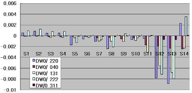
Figures 14 and 15 show the global wavefront coefficients depending on the lens radius error(Newton Ring=5) and thickness errors(50 μm), which indicates that the radius errors of surface S12 and S13 and the air gap (t12) between L6 and L7 are of high sensitivity. The main point is that the global wavefront coefficients by radius errors of surface S12 and S13 have the same sign with nearly the same amounts. It means, if the radius errors of S12 and S13 are arranged in the opposite direction, the optical system will have a small wavefront deformation. Also, If the air gap (t12) adopted a high precision spacer, it would be a relatively positive effect on performance.
By means of global wavefront coefficients on the lens manufacturing and assembly errors as in the way above, not only the effects of each element error on aberrations of an optical system, but also the size and direction of aberrations could be analyzed, which would contribute to finding out the way of minimizing aberrations and the proper compensation of aberrations.
Analyzing the tolerance of an optical system is mostly based on the tolerance in lens manufacturing and assembly, and the criterion regarding tolerance includes single values such as MTF, RMS wavefront error, and spot size. These methods, however, indicate neither how optical perturbations may cause aberrations to the optical system nor the correlation between such perturbations, and thus these cannot be the basis to enlarge the tolerance.
This paper introduced the global wavefront coefficients, which can indicate the aberration characteristics in every field regarding the small optical perturbation, and demonstrated that the optical system assembly structure and compensators can be accurately analyzed to maximize the tolerance based on the analysis of the size and direction of such coefficients. As the compensator to correct the distortion, we have showed that it is to be of high sensibility to distortion but all other aberrations. Also, the analysis above could lead to a way of compensating for a certain aberration or distortion based on the reaction between two elements. In addition, these analysis method will be very useful to analyze the tolerance for the environmental changes such as temperature or humidity.