Aircraft landing systems have been continuously developed because the landing phase is the most critical flight stage. According to Boeing’s statistical report, 59% of the commercial aircraft accidents occurred during the approach and landing phases although their flight time comprises only 16% of the total flight phase [1]. Moreover, 45% of the accidents were due to wind turbulences. Therefore, the landing controller should be robust enough for various disturbances such as wind turbulence, unpredictable gust near the ground, and control surface failures. In the conventional instrument landing system, the landing of the fixed-wing aircraft is divided into three phases: a glide phase, a flare phase, and a touchdown phase [2]. The aircraft approaches to the runway while tracking a specified glide slope in the glide phase and it follows an exponential path to slow the descent rate in the flare phase. VHF Omni Range (VOR) and radio beam are necessary to guide the aircraft to the pre-designed glide slope and runway. This system requires additional instruments in the aircraft to measure the signals that are transmitted from the ground system. Studies on the automatic landing controller have been performed recently by applying various control techniques: Proportional-Integral-Derivative (PID) control, Linear Quadratic Regulator (LQR),
The classical approaches of the landing controller use the PID control and the LQR for a linear model of the aircraft [2]. In order to deal with the uncertainties in the linear model, robust control techniques such as
The alternative approach to the model-based linear controller is a nonlinear adaptive control. In order to deal with the nonlinear aircraft model, feedback linearization and backstepping technique are considered [7,8]. Biju et al. designed a landing controller by using the feedback linearization [9]. Ju et al. developed a glide-slope tracking controller by using a non-adaptive backstepping technique [10]. However, in the nonlinear model highly nonlinear modeling errors and unknown parameter errors still exist. In order to deal with the uncertainties, various adaptive control theories are introduced: neural network, parameter adaptation, fuzzy logic, and genetic algorithm [11-16]. Saini et al. compared adaptive critic based neural networks with the PID controller in the aircraft landing [11]. Naikal et al. combined the classical landing controller with the radial basis function neural network [12]. Yoon et al. designed the backstepping controller to land the fixed-wing aircraft by using parameter adaptation [13]. Lee et al. compared the adaptive sliding mode controller with the feedback linearization in the landing of a quad-rotor [14]. Nho and Agarwal developed a fuzzy logic control system for the automatic landing of both linear and nonlinear aircraft models [15]. Ha modified the fuzzy logic controller through the optimization of the gain-scheduled controller by using a genetic algorithm in the automatic landing and touchdown flight [16].
In order to design the adaptive landing controller, wind disturbance and actuator failure near the ground should be considered. The wind disturbance increases the glideslope tracking error and it may cause a severe accident during the landing phase. In Ref. 12, the deterministic wind, wind turbulence, and wind-shear model are considered for the design of the landing controller. In Ref. 16, wind shear turbulence near the ground is modeled as head wind, crosswind, and downdraft, and the influence of the strong wind on the aircraft is analyzed. On the other hand, the probability of the actuator fault during the landing phase is higher compared to that during the cruise phase. This is due to the control surfaces of the aircraft which are commanded more rapidly and frequently during the landing phase. The actuator failure of the control surfaces during the landing phase causes more serious problem than during the cruise phase. These problems arise due to limited time and space for recovery. In Ref. 12, the actuator fault of multiple control surfaces is taken into account in the design of adaptive backstepping neural controller.
In this study, the automatic landing controller of the fixedwing aircraft is designed by using the backstepping scheme and the constrained adaptation technique. Nonlinear six degree-of-freedom aircraft model is considered for the design of the backstepping controller that tracks a desired glide slope toward the runway. In order to estimate the modeling errors of aerodynamic coefficients in the nonlinear model, the adaptive parameter estimation of the nonlinear function is adopted. The landing controller proposed in this study is different from the previous landing controllers in that the aggressive adaptation due to the wind disturbance and actuator failure is prevented by applying the hedging techniques. Even though the stability of the adaptive backstepping scheme is strictly addressed in the controller design, the dynamic characteristics of the system may cause an undesired behavior in the adaptive control. Moreover, each control surface of the aircraft has constraints which include magnitude saturation and rate limit. Therefore, the dynamic characteristics and the input constraints of the aircraft should be considered in the design of the adaptive control. In Ref. 17, a pseudo control hedging technique is proposed for the design of neural networks, and in Ref. 18, the pseudo control hedging is combined along with the training signal hedging techniques in the design of adaptive backstepping controller. In this study, the pseudo control hedging technique and the training signal hedging technique are combined with the command filter to design a reliable adaptive landing controller. In order to verify the landing performance of the constrained adaptive backstepping scheme, the glide-slope tracking errors of the constrained adaptive controller is compared with those of an unconstrained adaptive controller, a non-adaptive backstepping controller, and a gain-scheduled proportionalintegral controller. In numerical simulation, wind gust and actuator stuck during the landing phase are included for the evaluation of the landing performance.
The rest of this paper is organized as follows: Section 2 explains the landing procedure and the nonlinear dynamics of the fixed-wing aircraft. Section 3 describes the design of the adaptive backstepping controller by using the unconstrained and constrained adaptation schemes. In Section 4, nonlinear simulation result and analysis are presented. Conclusions are given in Section 5. In Appendix, the design procedure of the constrained adaptive backstepping controller is explained in detail.
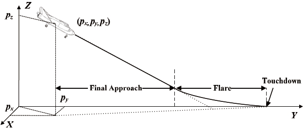
The automatic landing of the fixed-wing aircraft is divided into three phases: final approach, flare, and touchdown [19]. Figure 1 shows the conventional landing configuration of the fixed-wing aircraft. As shown in Fig. 1, (
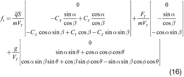
In this study, the six degree-of-freedom nonlinear dynamics of the fixed-wing aircraft is considered [2]. The force equations in the stability axis are represented as follows,
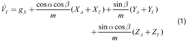
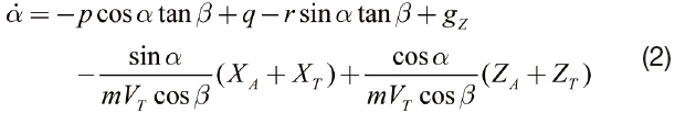
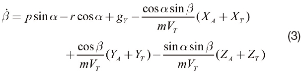
where,
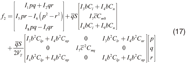
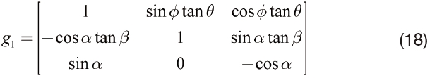
The moment equations are represented as follows,


where,
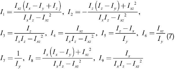
where,


Let us define the states


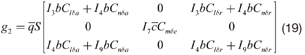
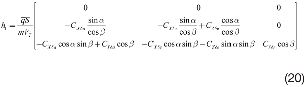
where, δa is an aileron control input, δe is an elevator control input, and δr is a rudder control input. By using the state and control input vectors which are defined in Eqs. (11)-(13), Eqs. (2)-(8) can be rewritten as,


where,
where,

is a dynamic pressure,

is a mean aerodynamic chord length,
3. Adaptive Backstepping Controller Design
3.1 Unconstrained Adaptive Backstepping Controller
In the design of the unconstrained adaptive controller, the dynamic characteristics and the input constraints of the aircraft are not considered. Figure 2 illustrates the schematic diagram of the unconstrained adaptive backstepping controller from the reference command


where,

and

are the estimation errors, and

and

are the estimates of

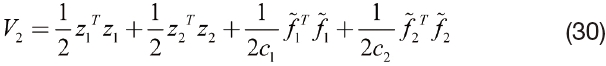
Consider the following Lyapunov function candidate
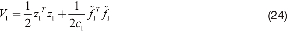
where,


where,
matrix. Therefore,
By substituting Eqs. (14), (21) and (23) into the time derivative of Eq. (24) yields,
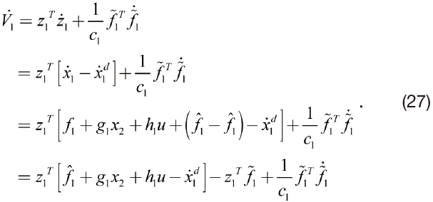
Applying Eqs. (25) and (26) to Eq. (27) yields

Therefore, the state error defined in Eq. (23) can be regulated, and

Consider the following Lyapunov function candidate
where,


where,
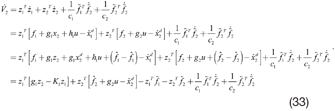
Finally, by applying Eqs. (26), (31), and (32) to Eq. (33) yields

In summary, the state errors defined in Eqs. (23) and (29) can be regulated. Therefore,
3.2 Constrained Adaptive Backstepping Controller
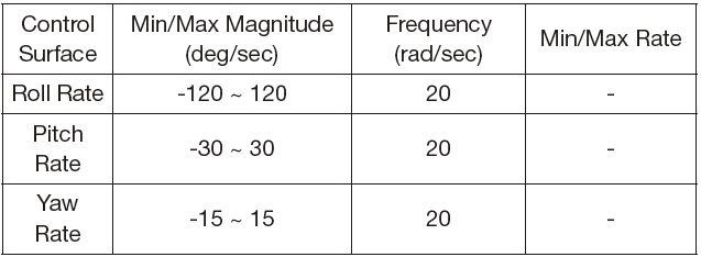
In the design of the constrained adaptive controller, the dynamic characteristics and the input constraints of the aircraft are considered. The desired state of Eq. (25) and the control input of Eq. (31) do not assure dynamic characteristics and constraints of the aircraft. In the adaptive controller, the desired states and/or control input may exceed the magnitude or the rate limitation if the dynamic characteristics of the states and the control input are not considered throughout the design procedure of the adaptation laws. These immoderate states or saturated control input may cause an aggressive adaptation in the adaptive laws of Eqs. (26) and (32). This can make the aircraft unstable or fly beyond the flight envelope. The command filter and the hedging techniques can deal with the dynamic characteristics and constraints such as response time, magnitude saturation, and rate limit [21- 24]. In Refs. 21 and 22, the adaptive controller is designed in the presence of the input saturation and constraints. Polycarpu et al. approximated the input saturation with the learning technique in the backstepping controller design [23]. Sonneveldt et al. designed the fault-tolerant flight controller by using the constrained adaptive backstepping scheme and neural networks [24]. Table 1 shows the dynamic characteristics of the actuator in the NASA HL-20 aircraft and it is considered in this study [25]. Table 2 shows the dynamic characteristics of the angular state in a general aircraft.
In this study, two techniques are applied to take the aggressive adaptation into account in the landing controller:
[Table 1.] Dynamic characteristics of control surface actuators (NASA HL-20)
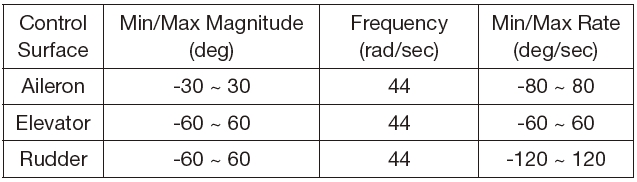
Dynamic characteristics of control surface actuators (NASA HL-20)
the command filter and the signal hedging. First, the command filter provides a filtered signal and its time derivative according to the desired dynamic characteristics. The command filter adopted in this study is a second-order nonlinear filter and it is defined as [18]
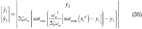
where,


where,
Second, compensating variables are introduced and the training signal and pseudo control hedging techniques are applied to prevent the estimation errors from aggressive adaptation. In the training signal hedging, the adaptation errors defined in Eqs. (36) and (37) are modified as follows [23].


where,

is the modified adaptation error,
[Table 2.] Dynamic characteristics of the aircraft angular rates
Dynamic characteristics of the aircraft angular rates
the desired state exceeds the filtered state, ξi reduces
until


In the same way, when

Finally, the desired virtual state in Eq. (25) and the desired control input in Eq. (31) are rewritten using

as follows,


It is to be noted that

is not the numerical derivative of
as follows,


Now, consider the following Lyapunov function candidate
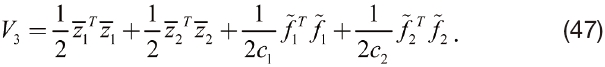
By substituting Eqs. (38)-(40) with
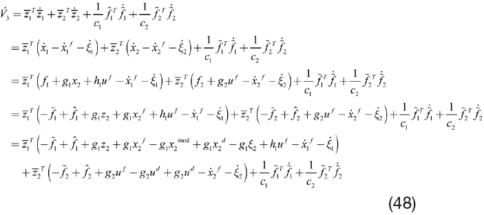
It is to be noted that the filtered state
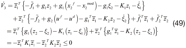
Finally, the time derivative of Eq. (47) is negative semidefinite. The state errors defined in Eqs. (38) and (39) are regulated. Therefore
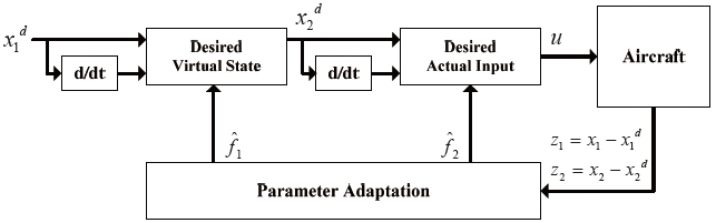
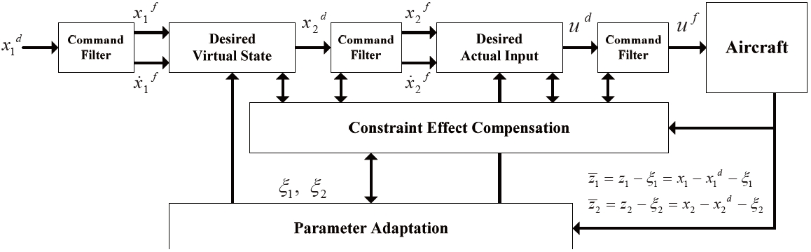
Figure 3 illustrates the schematic diagram of the constrained adaptive backstepping controller from the reference command
4. Simulation Result and Analysis
In order to verify the performance of the proposed control law, six degree-of-freedom nonlinear simulations are performed. The proposed constrained adaptive backstepping controller is compared with the gain-scheduled classical controller, the non-adaptive backstepping controller, and the unconstrained adaptive backstepping controller. The gainscheduled controller is designed by using Proportional-and-
Integral (PI) controller [26]. The non-adaptive backstepping controller is designed by assuming the estimation errors in Eqs. (21)-(22) zero and also by replacing f1 and f2 in Eqs. (25) and (31) with
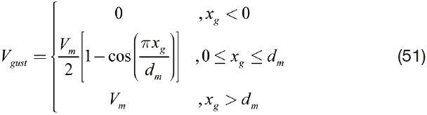
Wind gust and actuator fault are considered in the simulation of the NASA HL-20 model [25]. The NASA HL-20 simulation model contains WGS84 gravity model, COESA(Committee on Extension to the Standard Atmosphere) atmosphere model, and various wind models that include the wind shear model, the Dryden wind turbulence model, and the discrete wind gust model [25,26]. The wind shear model is implemented for the Category C terminal flight phase according to the Military Specification MIL-F-8785C. The magnitude of the shear wind is defined as follows,
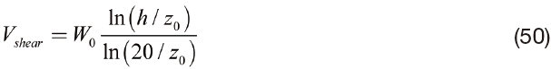
where,
where,
4.1 Simulation I: Wind Disturbance Case
The landing performance of each controller is compared to the case when the aircraft encounters an unknown wind gust. The glide slope is defined as a function of the range from the current position of the aircraft to the desired touchdown point [26]. The desired attitude of the aircraft along the glide slope is considered as follows,
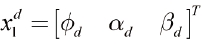
where, ød is a desired roll angle, αd is the desired angle of attack, and βd is the desired sideslip angle. The desired roll angle is generated for the regulation of the cross-range from the aircraft position to the runway center. The initial ød is zero because the aircraft is assumed to be aligned to the center of the runway at the start of the landing. βd is always kept to be zero. The initial condition of the aircraft is chosen as,

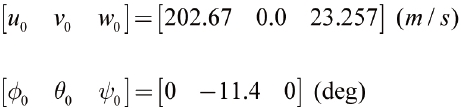
where, (
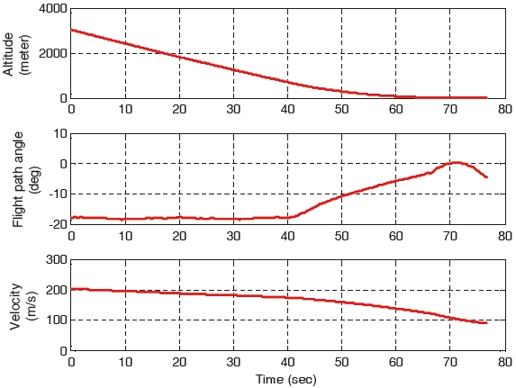
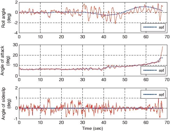
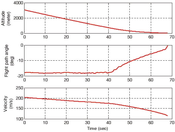
First, the wind turbulence is only considered and the wind gust is excluded. The landing performances of all the controllers are similar and they are as shown in Figs. 4-7. The control commands and the corresponding responses of the gain-scheduled PI controller and the constrained adaptive backstepping controller are shown in Figs. 4 and 5, respectively. The altitude, flight path angle, and the velocity of the aircraft are shown in Figs. 6 and 7, respectively.
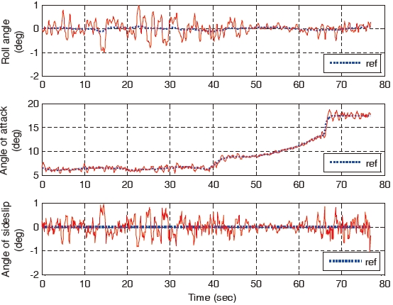
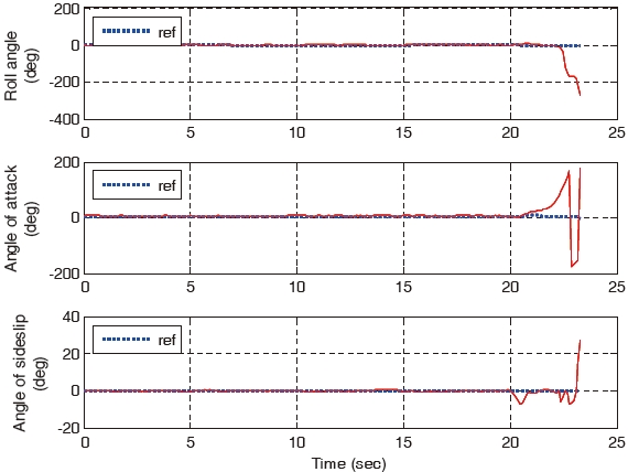
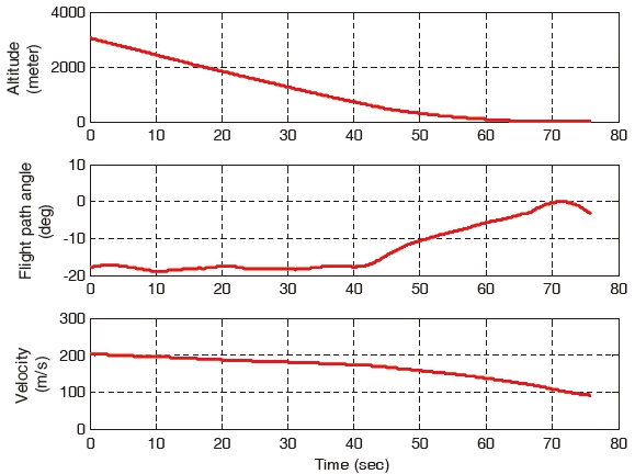
When the wind gust with a magnitude of 55 m/s is included in the simulation for 22 seconds, the tracking error
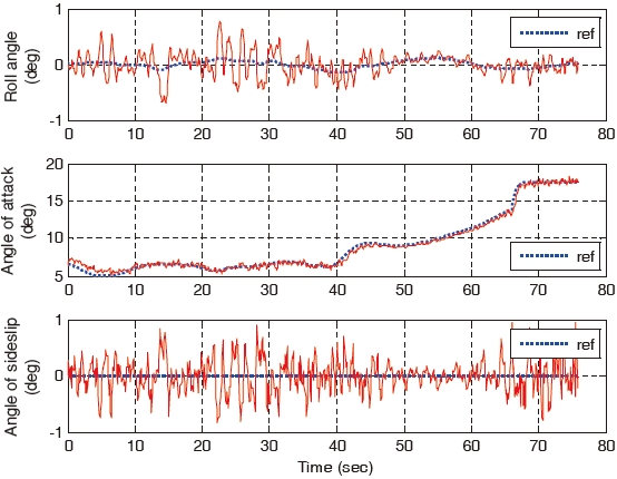
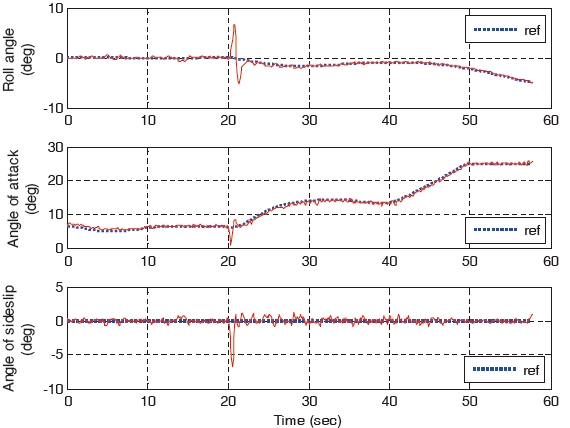
of the gain-scheduled PI controller increases. It is greater compared to that of the three backstepping controllers. The aircraft states of the gain-scheduled PI controller diverge at the final landing phase are as shown in Fig. 8. On the other hand, all the three backstepping controllers overcome the wind gust and they land successfully. This is as shown in Fig. 9. As shown in Fig. 8, the states diverge due to the pitch oscillation which cannot be stabilized in the gain-scheduled PI controller. On the other hand, the states do not diverge as a result of the parameter adaptation and constraint compensation in the constrained adaptive backstepping controller which is as shown in Fig. 9.
In order to compare the landing performance against the wind gust, a tracking performance index is defined as the following square sum of the tracking errors
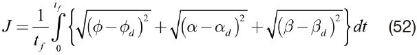
where,
[Table 3.] Comparison of the performance index according to the magnitude of wind gust

Comparison of the performance index according to the magnitude of wind gust
four controllers are similar. However, for the wind gust of magnitude greater than 16.5 m/s, the tracking error of the gain-scheduled PI controller increases steeply compared to that of the three backstepping controllers. The tracking error of the unconstrained adaptive backstepping controller is less than that of the non-adaptive backstepping controller when the magnitude of wind gust is smaller than 16.5 m/s because the small estimation errors in Eqs. (21) and (22) are well adapted. On the other hand, for the wind gust of magnitude greater than 16.5 m/s, the tracking error of the unconstrained adaptive backstepping controller is greater than that of the non-adaptive backstepping controller because of the large estimation error. This error occurs due to the wind gust which causes an overreacting adaptation. The non-adaptive backstepping controller provides an excellent tracking performance as long as the nonlinear functions
4.2 Simulation II: Actuator Stuck Case
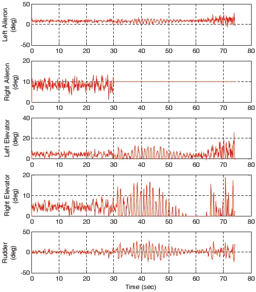
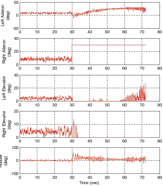
The landing performance of each controller is compared to the case where the aircraft encounters with an actuator fault. In this simulation, the actuator fault of the right aileron occurs during the landing phase. The right aileron is assumed to be stuck at a certain position. In this study, the fault detection and isolation logic of the control surface is not considered. Instead, the fault-tolerant performance of the proposed control law is evaluated to overcome the actuator stuck. In this simulation, the deflection angle of both the right and left ailerons is positive in the direction of trailing-edgedown, the deflection angle of the both right and left elevators is positive in the direction of trailing-edge-down, and the deflection angle of the rudder is positive in the direction of trailing-edge-left, respectively.
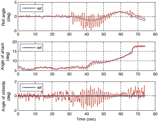
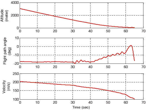
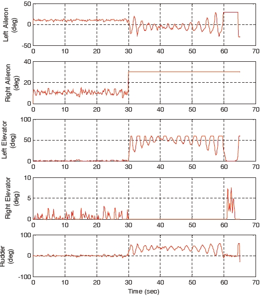
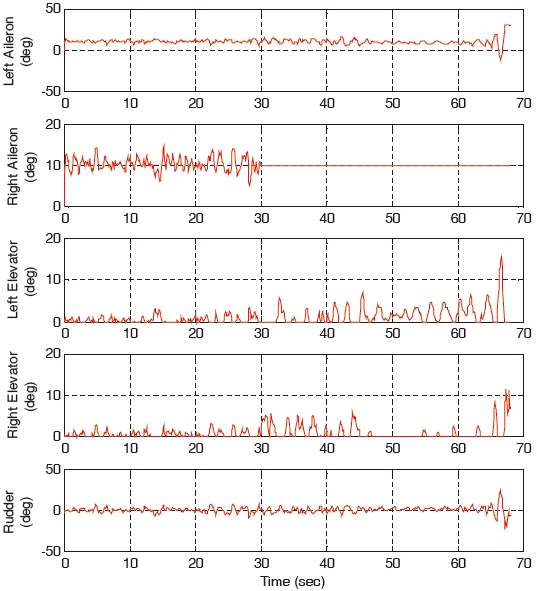
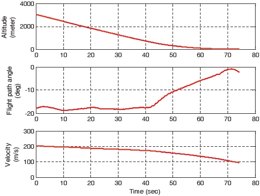
When the right aileron operating around 10°, is stuck at the position of 10° at 30 seconds, the landing performances of the gain-scheduled PI controller, the non-adaptive backstepping controller and the constrained adaptive backstepping controller are similar. The control responses, states, and control surfaces of the gain-scheduled PI controller are shown in Figs. 10, 11, and 12, respectively. Control responses, states, and control surfaces of the constrained adaptive backstepping controller are shown in Figs. 13, 14, and 15, respectively. As shown in Figs. 12 and 15, the angle of the right aileron is constant 10° after 30 seconds and this is due to the actuator stuck. Even though the right aileron is stuck, the aircraft that uses both the controllers tracks the glide slope successfully and it is as shown in Figs. 10 and 13.
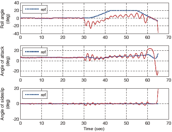
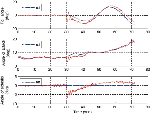
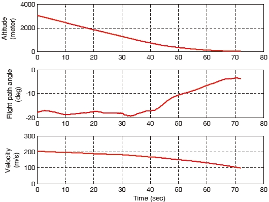
As the failure angle of the right aileron increases, the tracking error of the gain-scheduled PI controller becomes larger compared to the tracking errors of the constrained adaptive backstepping controller. When the right aileron is stuck at the position of 30° at 30 seconds, the aircraft landing of the gain-scheduled PI controller cannot be performed while the landings of the three backstepping controllers are successfully performed. The control responses, states, and control surfaces of the gain-scheduled PI controller when the stuck angle is 30° are shown in Figs. 16, 17, and 18, respectively. The control responses, states, and control surfaces of the constrained adaptive backstepping controller are shown in Figs. 19, 20, and 21, respectively. As shown in Figs. 18 and 21, the angle of the right aileron after 30 seconds is 30° and this is due to the actuator fault. As shown in Fig. 16, the aircraft of the gain-scheduled PI controller cannot track the roll angle command. As a result this tracking error causes a large error and an oscillation in tracking the angle-of-attack command. On the other hand, the aircraft of the constrained adaptive backstepping controller tracks the roll angle as well as the angle-of-attack commands. Finally, even though the right aileron is stuck it lands successfully on the runway.
In order to compare the landing performance against the actuator fault, the performance indices of the four controllers
[Table 4.] Comparison of the performance index according to the stuck angle of the right aileron
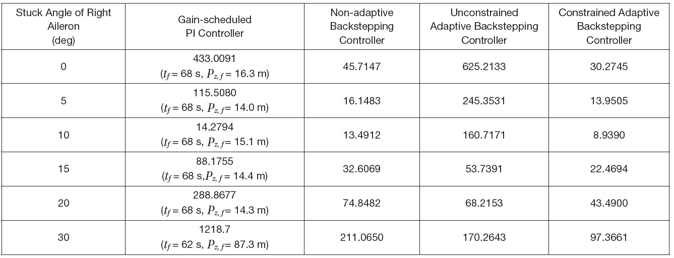
Comparison of the performance index according to the stuck angle of the right aileron
are summarized in Table 4. In all the cases, the right aileron was operating around 10° before the occurrence of the actuator stuck. As shown in Table 4, the tracking error of the gain-scheduled PI controller increases steeply as the stuck angle increases. This is due to the actuator fault which is not considered in the gain design process. The tracking error of the non-adaptive backstepping controller is less compared to that of the gain-scheduled PI controller even though the adaptation is not considered. The tracking error of the unconstrained adaptive backstepping controller is greater than that of the gain-scheduled PI controller for the stuck angle of 0, 5, and 10 deg, and it is greater than the tracking error of the non-adaptive backstepping controller for all the
cases. The poor performance of the unconstrained adaptive backstepping controller is due to the fact that the physical constraints of the control surfaces are not considered at all in the parameter adaptation. Unconstrained adaptation makes the system unstable and the situation worse. Finally, the tracking error of the constrained adaptive backstepping is the smallest for all the stuck angles and this is due to the parameter adaptation and the constraint compensation that is described in Eqs. (38)-(46).
Adaptive backstepping controller is designed to make the fixed-wing aircraft land on the runway in the presence of wind gust and actuator stuck. The nonlinear six degreeof- freedom dynamics of the aircraft is considered in the design of the backstepping controller. The adaptive scheme is applied to the backstepping controller in order to deal with the modeling errors in the aircraft dynamics and the external disturbances. In the parameter adaptation, the dynamic characteristics and the constraints of the aircraft states and actuator inputs are taken into account to prevent aggressive adaptation and provide a reliable landing. In order to verify the performance of the proposed control law numerical simulations are performed by using the nonlinear six degree-of-freedom aircraft model. The constrained adaptive backstepping controller successfully overcomes the wind gust and the actuator fault while the gain-scheduled PI controller, the non-adaptive backstepping controller, and the unconstrained adaptive backstepping controller cannot handle it.
The design procedure of the constrained adaptive backstepping controller is explained below in detail. With the command filter defined in Eq. (35), the nonlinear equations of aircraft motion are,


where,
Lemma 1. For the system of Eq. (A.1) with the adaptation error
are defined as


where,
Proof) Consider the following Lyapunov function candidate
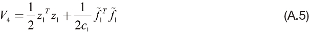
Substituting Eqs. (21), (36) and (A.1) into the time derivative of Eq. (A.5) yields
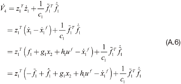
Applying Eqs. (A.3) and (A.4) to Eq. (A.6) yields
Lemma 2. For the system of Eqs. (A.1) and (A.2) that the filtered state does not exceed the desired state (

, and

are defined as


where,
Proof) Consider the following Lyapunov function candidate
Substituting Eqs. (21), (22), (36), (37), (A.1), and (A.2) into the time derivative of Eq. (A.12) yields
Applying Eqs. (A.8)-(A.11) to Eq. (A.13) yields
Lemma 3. For the system of Eqs. (A.1) and (A.2) that the filtered control input does not exceed the desired control input (
ξ1,
are defined as


Then, ξ1 converges to zero,
Proof) Consider the following Lyapunov function candidate
By substituting Eqs. (21), (22), (36), (37), (A.1), (A.2), and (A.15) into the time derivative of Eq. (A.19) yields,
By applying Eqs. (A.8), (A.11), (A.16), (A.17) and (A.18) to Eq. (A.20) yields,
Note that Eq. (A.9) is replaced with Eq. (A.17), and Eq. (A.10) is replaced with Eq. (A.18).
Theorem 1. For the system of Eqs. (A.1) and (A.2) that the filtered state and control input exceed the desired values (

ξ1, ξ2,
are defined as


Then, ξ1 and ξ2 converge to zero,
Proof) Consider the following Lyapunov function candidate
By substituting Eqs. (21), (22), (36), (37), (A.1), (A.2), (A.15), (A.22), and (A.25) into the time derivative of Eq. (A.27) yields,
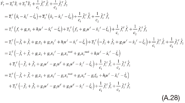
By applying Eqs. (A.8), (A.17), (A.18), (A.23), (A.24) and (A.26) to Eq. (A.28) yields,
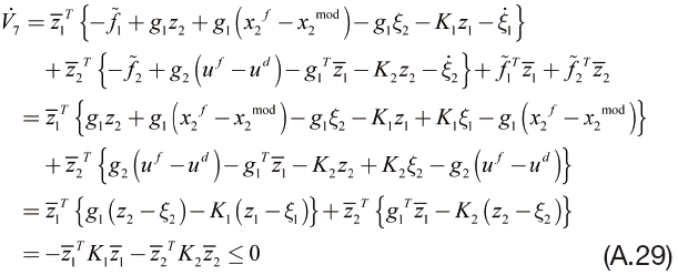
Note that Eqs. (A.9), (A.10), (A.11), and (A.16) are replaced with Eq. (A.17), (A.18), (A.26), and (A.23), respectively.