A rotary unmanned aerial vehicle (RUAV) can perform unique maneuvers such as hovering and vertical take-off and landing (VTOL). Recently, due to these characteristics, the demand of the RUAV development and utilization has seen unprecedented levels of growth not only in military but also in civilian applications. As a result of this trend, many researchers have carried out numerous works to deal with the control system design for the RUAV. However, as the RUAV is a multiple input multiple output (MIMO), unstable, underactuated and highly coupled system, the control system design of the RUAV is a challengeable work.

The control system of the RUAV is usually designed under the separation principle. This implies that the guidance and control subsystems are designed separately. The inner-loop SAS (Stability Augmentation System) and autopilots are designed to follow the commands that are generated by the outer-loop guidance algorithm, because the guidance loop has a much larger time constant compared to the inner-loop controller [1, 2]. In the design of the guidance loop, as the characteristics of the controller are not considered directly, the designed guidance loop may generate large control inputs that are hard on the control subsystems. Ignoring the coupling between the guidance and control loop may cause instability of the autopilot loop and/or the overall system. For this reason, a new guidance and control logic is proposed in this study by accounting for the physical relationship between the guidance and the control subsystems, especially for the RUAV.

In missile system, the separation principle of the guidance and control may not be valid especially when the missile is intercepting highly maneuverable target. This problem may be generated in the RUAV by highly nonlinear and coupled dynamics. To achieve improved performance for the case that the inner-loop autopilots cannot follow the acceleration commands generated by the guidance algorithm, many researchers have an interest in the integrated guidance and control (IGC) logic. Shima et al. applied a sliding method control (SMC) for the IGC design of the missile systems. Distance error was represented by using a line-of-sight (LOS) angle to integrate the guidance and control subsystems [3]. Menon et al. developed an integrated nonlinear missile guidance logic which considers the relative distance between rotating body frame and inertial frame, and applied feedback linearization and linear quadratic regulator [4-6].

In this study, the IGC scheme for the RUAV is proposed. First, the IGC model is derived taking into account the dynamic characteristics and the non-linear interaction between the kinematics and dynamics. The SMC scheme is applied to design the guidance and control law of the RUAV. Moreover, slack variable is introduced to deal with the under-actuated problem of the RUAV. The performance of the proposed IGC law was evaluated and it was compared with the conventional separated guidance and control (SGC) law through numerical simulations. The contribution of this paper is to make the system more robust against uncertainties such as external disturbance and parameter variation. As a result, the RUAV can effectively exhibit high maneuvering by using less control input. It is less susceptible to the saturation and stability problems. It can be concluded that the proposed IGC method overcomes the shortcomings of the conventional approaches.

This paper is organized as follows. Section 2 presents the linear model of the RUAV, nonlinear kinematics in the guidance problem, and the IGC model. Section 3 describes the IGC controller design process which considers the SMC and slack variable. Section 4 provides the performance evaluation results of the IGC system by conducting numerical simulations for several missions. Finally, concluding remarks and further research works are addressed in Section 5.

The linear model of the RUAV considered in this study can be written as follows,

Where,

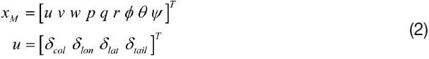
The state vector denotes the velocity components (u, v, w) with respect to the X-Y-Z axis of the body coordinate frame, the corresponding angular rates (p, q, r), and the Euler angles (ø, θ, ψ). The control input vector denotes the inputs to the main rotor collective pitch, the longitudinal cyclic pitch, the lateral cyclic pitch, and the tail rotor collective pitch [7].

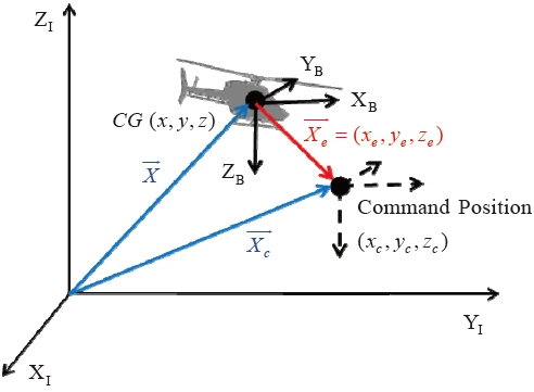
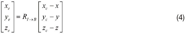
Let us consider a flight situation of the RUAV approaching the desired command position as shown in Fig. 1. There are two coordinate frames: inertial coordinate frame (X_I, Y_I, Z_I) , and body coordinate frame (X_B, Y_B, Z_B) . The guidance error states to derive the IGC model is chosen as,

Where, (x_e, y_e, z_e) denotes the position errors between the mass center of the RUAV (x, y, z) and the command position (x_c, y_c, z_c). In this study, (x, y, z) and (x_c, y_c, z_c) are defined in the inertial coordinate frame, while (x_e, y_e, z_e) is defined in the body frame. Thus, (x_e, y_e, z_e) can be represented as,

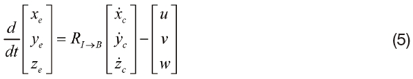
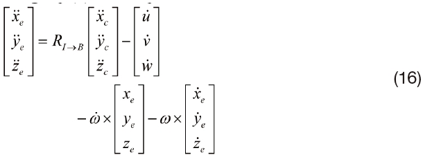
Differentiating Eq. (4) with respect to time yields,

By using the transport theory, the derivative of (x_e, y_e, z_e) can be obtained as,

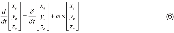
Where,

and

are the time derivatives with respect to the inertial frame and the body frame, respectively, and ω = [p q r]. From Eq. (5) and Eq. (6), the time derivative of (x_e, y_e, z_e) in the body frame can be obtained as follows,

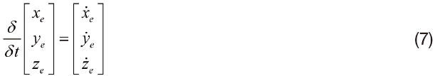
The above equation provides the first time derivative of the kinematic equation that is related to the guidance states. Note that a superscription, ’ · ’, is used when a vector is differentiated with respect to time in the frame that the vector is defined. Let us define (ø_e, θ_e, ψ_e) as the attitude error angle between the Euler angle and the command angle (ø_c, θ_c, ψ_c).

In order to determine the command angles, the following relationship between the acceleration of the RUAV mass center and external force that acts on the RUAV is considered.

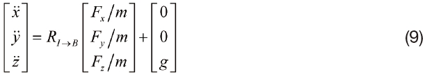
Where, (F_x, F_y, F_z) are the elements of the total aerodynamic force vector along the body coordinate frame, m is the mass of the RUAV, and g is the gravitational acceleration, respectively. In Eq. (9),

is regarded as a set of pseudo control variables, (v_x, v_y, v_z) and they can be achieved as,

By substituting the pseudo control inputs into the acceleration terms in Eq. (9), the desired values of the roll and pitch attitude angles among the Euler angles can be computed. In this process, two approximations are used to simplify the computations. First, it is assumed that the forces generated by the cyclic and tail rotor collective stick inputs are relatively smaller compared to the force and this is due to the main rotor collective stick input. Thus, (F_x, F_y, F_z) can be approximated as

and this is related only to the main rotor collective stick input. Second,

and

are assumed to be much smaller than

Hence, in Eq. (9) they are negligible.

Then, the command roll and pitch attitude angles can be approximated as follows,

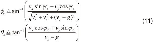
Where, ψ_c is the command yaw attitude angle which can be determined as,

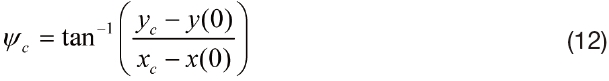
In Eq. (12), x(0) and y(0) are the x and y directional initial position of the RUAV along the inertial coordinate frame [8, 9]. In general, the RUAV does not ascend sharply with the acceleration of 1g [m/s2]. Therefore, the singularity problem of this case is not considered in Eq. (11). Moreover, two cases are examined to avoid the singularity in Eq. (12). First, if both x_c ？ x(0) ？ 0 and y_c ? y(0) ？ 0 are hold then, the hovering flight maneuver is generated to maintain the current yaw attitude angle. Second, if x_c ? x(0) ？ 0 and y_c ? y(0) ≠ 0 then , 90 degrees is generated for the yaw angle command.

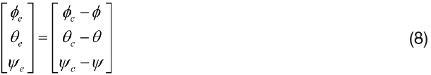
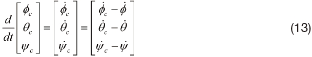
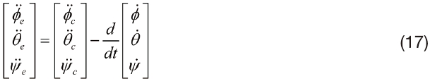
On the other hand, the time derivative of the attitude error angle can be simply obtained by differentiating Eq. (8) with respect to time as,

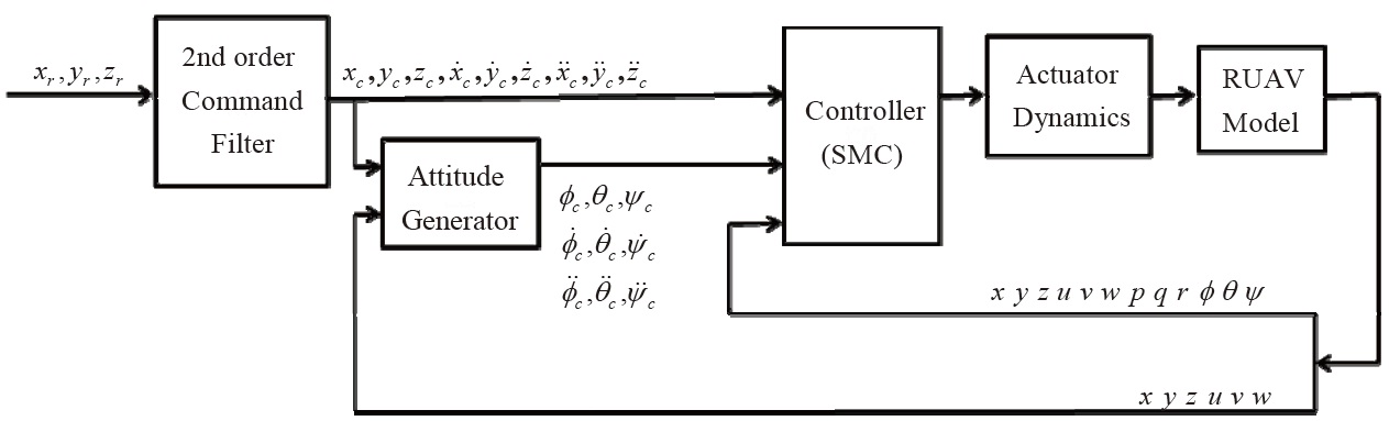
In this study, it is assumed that the first and second time derivatives of command positions and angles can be obtained by using the second-order command filter [10].

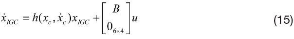
Now, let us derive the equations of the total IGC system. The state vector of the IGC model is defined by,

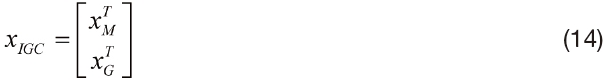
The equations of motion can be obtained by using Eqs. (7) and (13) as,

It is to be noted that the second-order actuator dynamics is used to consider the response of the control surfaces. The overall system block diagram is shown in Fig. 2.

In this section, the SMC is designed to construct the control inputs for the IGC model. The SMC is well known as a robust control design method, and it is suitable to treat nonlinear systems with large modeling errors, uncertainties, and disturbances.

The SMC makes the guidance error states to converge to zero values. In order to find out the relationship between the control inputs and the guidance states, the second order derivatives of the guidance states are derived.

By differentiating Eq. (7) with respect to time yields,

Differentiating Eq. (13) with respect to time yields,

In order to determine the second term on the right-hand side of Eq. (17), let us consider the differential equation that relates to the angular rates (p, q, r) with the Euler angles (ø, θ, ψ) [1].

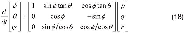
Finally, by using Eqs. (16) and (17), the second time derivative equations of the guidance states are derived as,

Where, f ∈ R^6×1 and g ∈ R^6×4.

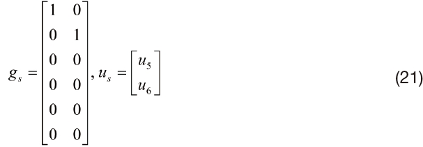
The RUAV is an under-actuated system. Therefore, g of Eq. (19) is a 6-by-4 matrix and not invertible. In this study, the

slack variable approach is adopted to design the available control inputs. By augmenting the slack variable g_s to g and u_s to u in order to form a square matrix, the control inputs can be determined. In this process, Eq. (19) can be represented as,

Where,

The slack variable g_s is introduced to make the matrix G invertible, and u_s can be adopted as,

Then, we have

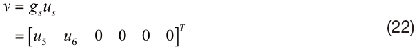
Note that the slack variables u₅ and u₆ should be estimated [11].

Now, let us define the SMC sliding surface as,

Where, K₁ is a diagonal matrix with positive entries. It is intended that the IGC system operates on the SMC sliding surface, which is defined as s = 0. The control inputs are designed by using the following Lyapunov candidate function.

Where,

is defined as,

Note that

is the estimated value of v, and

can be represented as

with an assumption that v changes slowly. Then, the time derivative of the Lyapunov candidate function can be derived as,

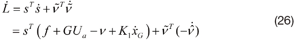
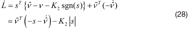
According to the Lyapunov stability theorem, the augmented control inputs are designed to make the time derivative of the Lyapunov candidate function as negative semi-definite. The control inputs are chosen as,

Where, K₂ is an input gain (diagonal) matrix which has positive entries. By substituting the augmented control inputs of Eq. (27) into the time derivative of the Lyapunov candidate function of Eq. (26) yields,

Let us update the estimated value

as,

Then, the time derivative of the Lyapunov candidate function can be represented as,

As the time derivative of the Lyapunov candidate function is negative semi-definite, it can be concluded that the SMC sliding surface s = 0 of Eq. (23) is reached in a finite time. This implies that the regulation of the guidance states can be achieved in a finite time.

In this section, two cases of numerical simulations are performed to verify the performance of the proposed IGC scheme. The first simulation scenario is waypoint guidance. In order to test the robustness of IGC scheme, the second simulation scenario includes a constant wind disturbance. The simulation results of the IGC are compared with the conventional separated guidance and control (SGC) scheme. In order to design the controller of the SGC scheme, the output feedback linear quadratic (LQ) tracker is used [12].

Simulations are carried out by using MATLAB Simulink. Moreover, the RUAV model is based on the X-Cell 60 SE helicopter which was identified by MIT. In this study, the ground effect and the sensor noise are not considered. In order to reduce the chattering phenomenon caused by sign function, sgn(s), hyperbolic tangent function is used instead of the sign function. Parameters for the simulations are selected as follows,

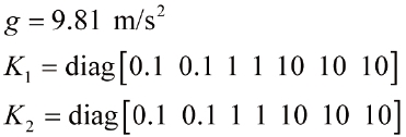
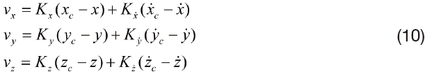
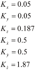
Control gains for pseudo control variables in Eq. (10) are designed as,

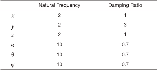
The gains of the second order command filter for each X-Y-Z axis position and the Euler angles (ø, θ, ψ) are summarized in Table 1.

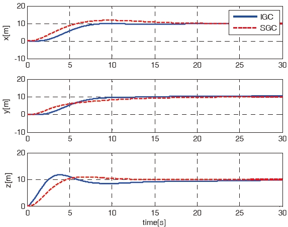
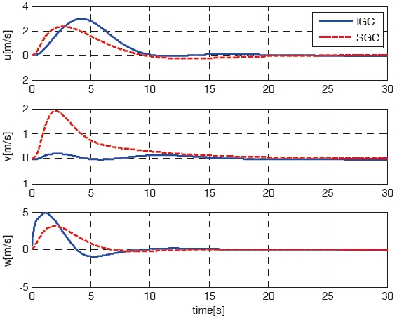
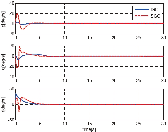
For the first case, the mission of the RUAV is a forward flight from origin (0, 0, 0) to the goal point (10, 10, 10). The simulation results using the IGC scheme are compared with the results using the SGC scheme. Figures 3 - 7 shows the simulation results of the IGC and SGC schemes, respectively. Figure 3 shows the X-Y-Z axis position histories of the RUAV for the IGC and SGC schemes. As shown in Fig. 3, the RUAV approaches to the goal point well for both the schemes. Figures 4 - 6 show the velocities, the attitude angles, and the

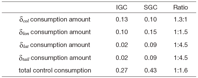
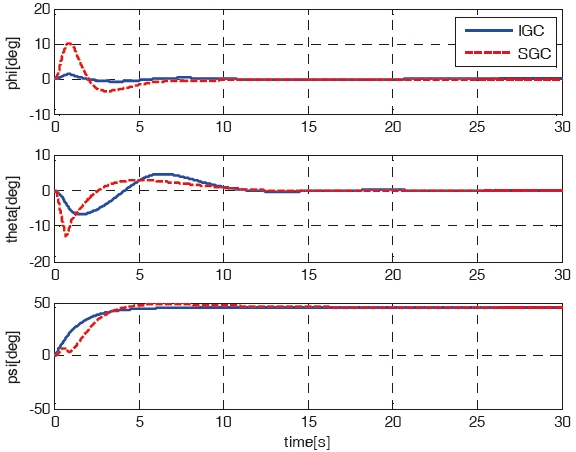
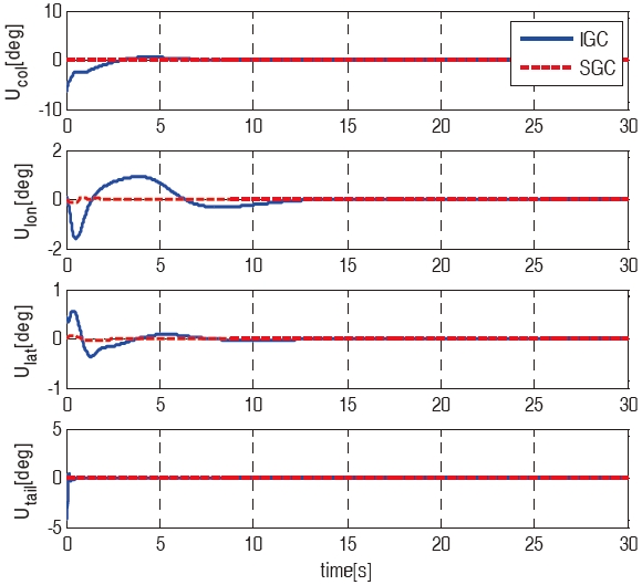
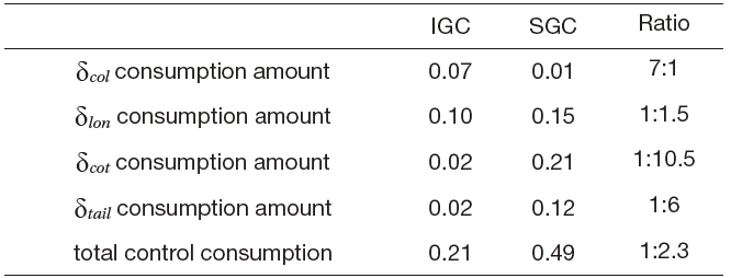
angular rates of the IGC and SGC schemes. As shown in Figs. 5 and 6, the SGC scheme shows a tendency to have much more oscillations, and a slower convergence time compared to those of the IGC scheme. Figure 7 shows the time histories of the control inputs. Table 2 summarizes the consumed control inputs of each scheme. The amount of control consumption is computed by using the following measure.

Even though both the IGC and SGC schemes have similar position tracking performances, the SGC scheme consumes about 1.5 times as much control input as the IGC scheme.

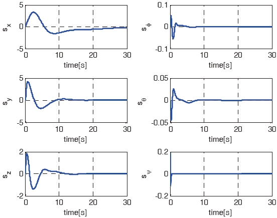
In conclusion, the simulation results show that the IGC scheme improves the performance of the RUAV. Figure 8 shows that the SMC surfaces converge to zero. By this result, it can be stated that the IGC system is well controlled.

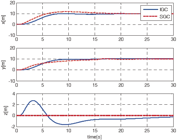
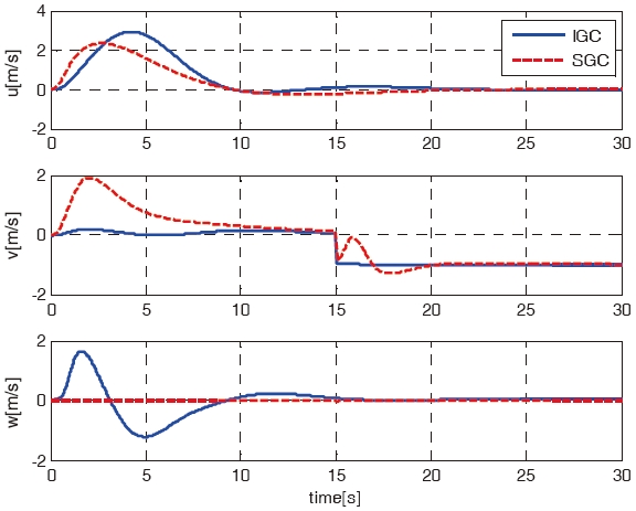
For the second case, the forward flight mission is given to the RUAV from the origin (0, 0, 0) to the goal point (10, 10, 0). In this case, constant wind disturbance is considered and it is assumed to be blown along the Y-axis in the body frame with -1 m/s at 15 sec. Figures 9 - 13 show the results of the IGC and SGC schemes, respectively. Figures 9 and 10 show the X-Y-Z axis position histories and velocity histories of the RUAV for the IGC and SGC schemes. As shown in Fig. 9, the RUAV approaches to the goal point well regardless of the wind disturbance for both the schemes. Figure 10 shows

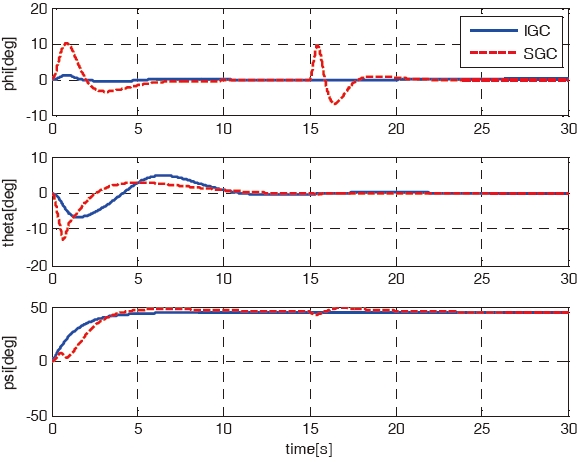
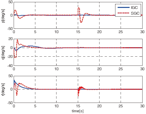
the influence of constant wind disturbance at 15 sec. Figures 11 and 12 show the attitude angles and the angular rates of the IGC and SGC schemes. As shown in the figures, due to the wind disturbance along the Y-axis, the longitudinal attitudes of both the schemes are affected. However, as shown in Figs. 11 and 12, the SGC scheme is disturbed more harshly compared to the IGC scheme. Especially, the maximum magnitude of roll attitude angle of SGC is about 10

degrees at 15 sec while that of the IGC is close to zero. These simulation results demonstrate that the SGC compared to IGC, has more unstable bank motion to perform a complex maneuver. If a more complex flight mission is needed then,

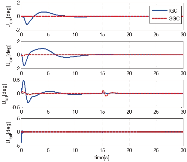
the SGC scheme may not achieve it. Figure 13 shows the time histories of the control inputs. Table 3 summarizes the consumed control inputs of the IGC and SGC schemes. The SGC method consumes about 2 times as much control input as the IGC method.

In conclusion, the simulation results show that the IGC scheme is more robust to the disturbance compared to the SGC scheme.

The IGC scheme is proposed and applied to the RUAV. In order to derive the RUAV model for the IGC, the dynamics of RUAV and kinematics that is related with guidance are integrated. The sliding mode controller augmented with the slack variables is used for the design of the IGC system. Numerical simulations are performed for the two missions. The first case is waypoint guidance. In the second case, in order to verify the robustness of the IGC system, a constant wind disturbance is considered. The simulation results of the IGC scheme are compared with those of the conventional SGC scheme. The simulation results showed that the proposed scheme gives better performances compared to the conventional method. In other words, the IGC scheme provides fast response as well as robustness with respect to the external disturbance, and it consumed less control input.

As a future work, the nonlinear model of RUAV should be considered in the design of the IGC system. Moreover, for better guidance and control performance of the IGC system, other nonlinear controllers such as feedback linearization and backstepping techniques are to be better considered. Finally, a flight test by using an embedded system mounted

on the performance RUAV should be performed to verify the performance of the proposed IGC scheme.