This paper presents an advanced computational method for the prediction of the responses in the frequency domain of general linear dissipative structural-acoustic and fluid-structure systems, in the low-and medium-frequency domains and this includes uncertainty quantification. The system under consideration is constituted of a deformable dissipative structure that is coupled with an internal dissipative acoustic fluid. This includes wall acoustic impedances and it is surrounded by an infinite acoustic fluid. The system is submitted to given internal and external acoustic sources and to the prescribed mechanical forces. An efficient reduced-order computational model is constructed by using a finite element discretization for the structure and an internal acoustic fluid. The external acoustic fluid is treated by using an appropriate boundary element method in the frequency domain. All the required modeling aspects for the analysis of the medium-frequency domain have been introduced namely, a viscoelastic behavior for the structure, an appropriate dissipative model for the internal acoustic fluid that includes wall acoustic impedance and a model of uncertainty in particular for the modeling errors. This advanced computational formulation, corresponding to new extensions and complements with respect to the state-of-the-art are well adapted for the development of a new generation of software, in particular for parallel computers.
aijkh = elastic coefficients of the structure
bijkh = damping coefficients of the structure
c0 = speed of sound in the internal acoustic fluid
cE = speed of sound in the external acoustic fluid
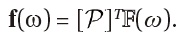
f = vector of the generalized forces for the internal acoustic fluid
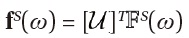
fS = vector of the generalized forces for the structure
g = mechanical body force field in the structure
i = imaginary complex number i
k = wave number in the external acoustic fluid
n = number of internal acoustic DOF
ns = number of structure DOF
nj = component of vector n
n = outward unit normal to ∂Ω
nsj = component of vector nS
nS = outward unit normal to ∂ΩS
p = internal acoustic pressure field
pE = external acoustic pressure field
pE|ΓE = value of the external acoustic pressure field on ΓE
pgiven = given external acoustic pressure field
pgiven|ΓE = value of the given external acoustic pressure field on ΓE
q = vector of the generalized coordinates for the internal acoustic fluid
qS = vector of the generalized coordinates for the structure

= component of the damping stress tensor in the structure
t = time
u = structural displacement field
v = internal acoustic velocity field
xj = coordinate of point x
x = generic point of R3
[A] = reduced dynamical matrix for the internal acoustic fluid
[A] = random reduced dynamical matrix for the internal acoustic fluid

= dynamical matrix for the internal acoustic fluid
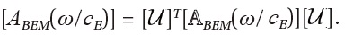
[ABEM] = reduced matrix of the impedance boundary operator for the external acoustic fluid

= matrix of the impedance boundary operator for the external acoustic fluid
[AFSI] = reduced dynamical matrix for the fluid-structure coupled system
[AFSI] = random reduced dynamical matrix for the fluid-structure coupled system

= dynamical matrix for the fluid-structure cou
[AS] = reduced dynamical matrix for the structure
[AS] = random reduced dynamical matrix for the structure

= dynamical matrix for the structure
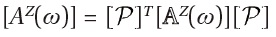
[AZ] = reduced dynamical matrix associated with the wall acoustic impedance

= dynamical matrix associated with the wall acoustic impedance
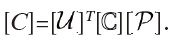
[C] = reduced coupling matrix between the internal acoustic fluid and the structure
[C] = random reduced coupling matrix between the internal acoustic fluid and the structure

= coupling matrix between the internal acoustic fluid and the structure
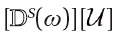
[D] = reduced damping matrix for the internal acoustic fluid
[D] = random reduced damping matrix for the internal acoustic fluid

= damping matrix for the internal acoustic fluid
[DS] = reduced damping matrix for the structure
[DS] = random reduced damping matrix for the structure

= damping matrix for the structure
DOF = degrees of freedom

= vector of discretized acoustic forces

= vector of discretized structural forces
Gijkh(0) = initial elasticity tensor for viscoelastic material
Gijkh(t) = relaxation functions for viscoelastic material
G = mechanical surface force field on ∂Ωs
[G] = random matrix
[G0] = random matrix
[K] = reduced “stiffness” matrix for the internal acoustic fluid
[K] = random reduced “stiffness” matrix for the internal acoustic fluid

= “stiffness” matrix for the internal acoustic fluid
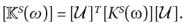
[KS] = reduced stiffness matrix for the structure
[KS] = random reduced stiffness matrix for the structure

= stiffness matrix for the structure
[M] = reduced “mass” matrix for the internal acoustic fluid
[M] = random reduced “mass” matrix for the internal acoustic fluid

= “mass” matrix for the internal acoustic fluid
[MS] = reduced mass matrix for the structure
[MS] = random reduced mass matrix for the structure

= mass matrix for the structure

= internal acoustic mode
[P] = matrix of internal acoustic modes
Q = internal acoustic source density
QE = external acoustic source density
Q = random vector of the generalized coordinates for the internal acoustic fluid
QS = random vector of the generalized
P = random vector of internal acoustic pressure DOF

= vector of internal acoustic pressure DOF
U = random vector of structural displacement DOF

= vector of structural displacement DOF

= elastic structural mode α
[u] = matrix of elastic structural modes
Z = wall acoustic impedance
ZΓE = impedance boundary operator for external acoustic fluid
δ = dispersion parameter
εkh = component of the strain tensor in the structure
ω = circular frequency in rad/s
ρ0 = mass density of the internal acoustic fluid
ρE = mass density of the external acoustic fluid
ρS = mass density of the structure
σ = stress tensor in the structure
σij = component of the stress tensor in the structure

= component of the elastic stress tensor in the structure
τ = damping coefficient for the internal acoustic fluid
∂Ω = boundary of Ω
∂ΩE = boundary of ΩE equal to ΓE
∂ΩS = boundary of Ωs
Γ = coupling interface between the structure and the internal acoustic fluid
ΓE = coupling interface between the structure and the external acoustic fluid
ΓZ = coupling interface between the structure and the internal acoustic fluid with acoustical properties
Ω = internal acoustic fluid domain
Ωi =

(ΩE?ΓE)
ΩE = external acoustic domain
ΩS = structural domain
The fundamental objective of this paper is to present an advanced computational method for the prediction of the responses in the low-and medium-frequency domains of general linear dissipative structural- acoustic and fluid-structure systems. The system under consideration is constituted of a deformable dissipative structure and it is coupled with an internal dissipative acoustic fluid which includes wall acoustic impedances. The system is surrounded by an infinite acoustic fluid and it is submitted to a given internal and external acoustic sources and to the prescribed mechanical forces.
Instead of presenting an exhaustive review of such a problem in this introductory section, we have preferred to move on to the review discussions in each relevant section.
Concerning the appropriate formulations for computing the elastic, acoustic and elastoacoustic modes of the associated conservative fluid-structure system, including substructuring techniques, for the construction of the reduced-order computational models in fluid-structure interaction and for structural-acoustic systems, refer to Ref. [1-5]. For the dissipative complex systems, readers can find out the details of the basic formulations in Ref. [3].
In this paper, the proposed formulation that corresponds to new extensions and complements with respect to the state-of-the-art can be used for the development of a new generation of computational software in particular to the context of parallel computers. We present here an advanced computational formulation. This is based on an efficient reduced-order model in the frequency domain and for this all the required modeling aspects for the analysis of the medium-frequency domain have been taken into account. To be more precise, we have introduced a viscoelastic modeling for the structure, an appropriate dissipative model for the internal acoustic fluid that includes wall acoustic impedance and finally, a global model of uncertainty. It should be noted that model uncertainties must be absolutely taken into account in the computational models of complex vibroacoustic systems in order to improve the prediction of responses in the medium-frequency range. The reduced-order computational model is constructed by using finite element discretization for the structure and for the internal acoustic fluid.
The external acoustic fluid is treated by using an approximate boundary element method in the frequency domain.
The sections of the paper are:
1. Introduction
2. Statement of the problem in the frequency domain
3. External inviscid acoustic fluid equations
4. Internal dissipative acoustic fluid equations
5. Structure equations
6. Boundary value problem in terms of {u, p}
7. Computational model
8. Reduced-order computational model
9. Uncertainty quantification
10. Symmetric boundary element method without spurious frequencies for the external acoustic fluid
11. Conclusion
References are given at the end of the paper.
2. Statement of the Problem in the Frequency Domain
We consider a mechanical system made up of a damped linear elastic free-free structure Ω
We are interested in the responses in the
to
The physical space

is referred to a cartesian reference system and we denote the generic point of
by x = (


in which the circular frequency ω is real. Nevertheless, for other quantities some exceptions to this rule are done and in such a case, the Fourier transform of a function


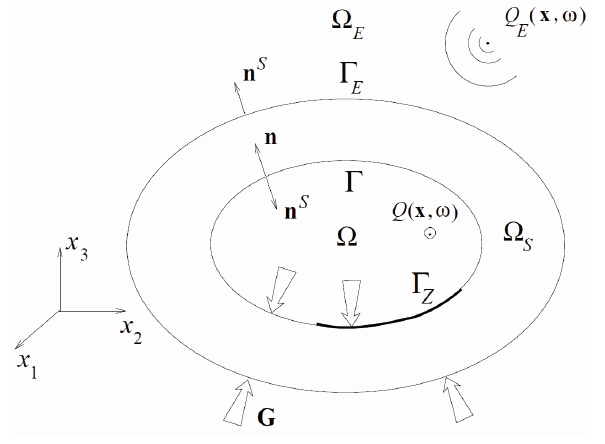
2.2 Geometry -Mechanical and acoustical hypotheses Given loadings
The coupled system is assumed to be in linear vibrations around a static equilibrium state and this is taken as a natural state at rest.
Structure Ω
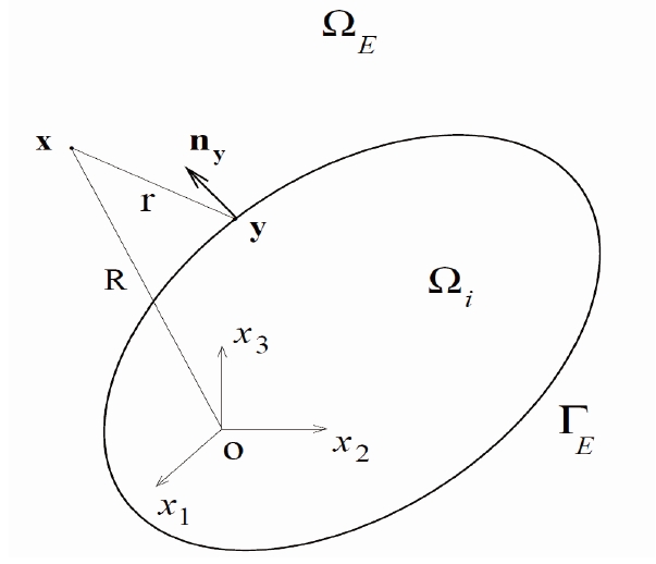
The structure at the equilibrium occupies the three-dimensional bounded domain Ω
(see Fig. 2). The displacement field in Ω
Internal dissipative acoustic fluid Ω. Let Ω be the internal bounded domain that is filled with a dissipative acoustic fluid (gas or liquid) as described in Section 4. The boundary ∂Ω of Ω is Γ?Γ
External inviscid acoustic fluid Ω
Note that in general, Ω
3. External Inviscid Acoustic Fluid Equations
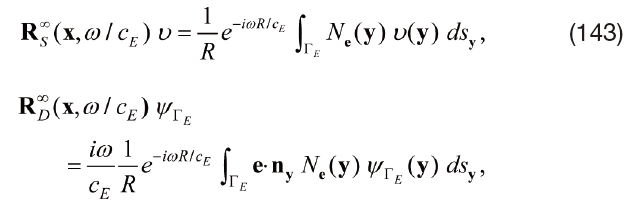
An inviscid acoustic fluid occupies an infinite domain Ω

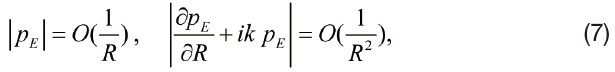
with

in which the different quantities are defined in Section 10. This is a self-contained section that describes the computational modeling of the external inviscid acoustic fluid by an appropriate boundary element method. It should be noted that in Eq. (8), the pressure field
4. Internal Dissipative Acoustic Fluid Equations
4.1 Internal dissipative acoustic fluid equations in the frequency domain
The fluid is assumed to be homogeneous, compressible and dissipative. In the reference configuration, the fluid is at rest. The fluid is either a gas or a liquid and the gravity effects are neglected (see Ref. [9] to take into account both gravity and compressibility effects for an inviscid internal fluid). Such a fluid is called as a
The dissipation due to thermal conduction is neglected and the motions are assumed to be irrotational. Let, ρ0 be the mass density and


τ is given by,
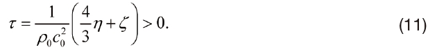
The constant
Taking
4.2 Boundary conditions in the frequency domain
(i) Neumann boundary condition on Γ. By using Eq. (10) and v·n =
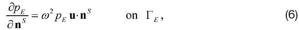
(ii) Neumann boundary condition on Γ

Wall acoustic impedance
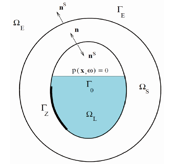
4.3 Case of a free surface for a liquid
Cavity Ω is partially filled with a liquid (dissipative acoustic fluid) that occupies the domain Ω

5.1 Structure equations in the frequency domain
The equation of the structure that occupies the domain Ω

in which ρs(x) is the mass density of the structure. The constitutive equation (linear viscoelastic model, see Section 5.2, Eq. (31)) is such that the symmetric stress tensor σ

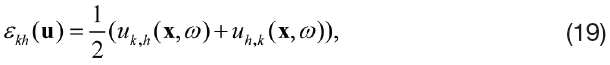
in which the symmetric strain tensor
and where the tensors

in which
As n

in which
5.2 Viscoelastic constitutive equation
In dynamics, the structure must always be modeled as a dissipative continuum. For the conservative part of the structure, we use the linear elasticity theory which allows the structural modes to be introduced. This was justified by the fact that in the low-frequency range, the conservative part of the structure can be modeled as an elastic continuum. In this section, we introduce damping models for the structure that is based on the general linear theory of viscoelasticity and it is presented in Ref. [15] (see also Ref. [16,17]). Complementary developments are presented with respect to the viscoelastic constitutive equation detailed in Ref. [3].
In this section, x is fixed in Ω

as

Constitutive equation in the time domain. The stress tensor
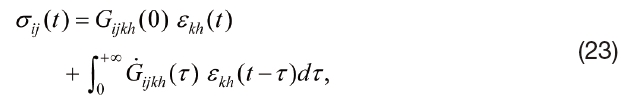
Where,

has the usual property of symmetry and

and are assumed to be integrable on [0, +∞[. Functions

Therefore, the limit of

The tensor
For all x that is fixed in Ω
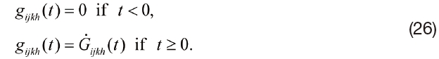
As
By using Eq. (26), Eq. (23) can be rewritten as,
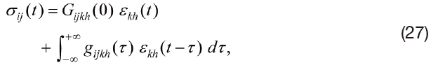
It should be noted that Eq. (27) corresponds to the most general formulation in the time domain within the framework of the linear theory of viscoelasticity. The usual approach which consists in modeling the constitutive equation in time domain by a linear differential equation in
Constitutive equation in the frequency domain. The general constitutive equation in the frequency domain is written as,

in which,


Equation (28) can then be rewritten as,

Tensors


and the positive-definiteness properties, i.e., for all the second-order real symmetric tensors


in which the positive constants
As

is defined by,
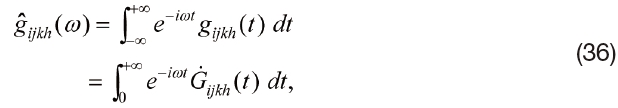
and it is a complex function which is continuous on ]?∞, +∞[ and such that

The real part
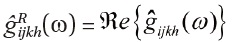
and the imaginary part
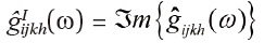
of
are even and odd functions. So, it is easy to say that
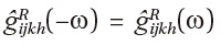
and
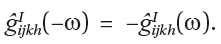
We can then deduce that

We can now take the Fourier transform of Eq. (27) and using Eq. (31) yields the relations,


Eqs. (37), (39) and (40) yields,


From Eqs. (31), (41) and (42), we deduce that

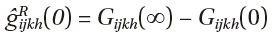
Eq. (43) shows that viscoelastic materials behave elastically at high frequencies with elasticity coefficients that are defined by the initial elasticity tensor

As pointed out before, a positive-definite tensor

in which σ

The reader should be aware of the fact that the constitutive equation of an elastic material in a static deformation process is defined by
is a negative- definite tensor.
As

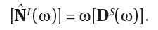
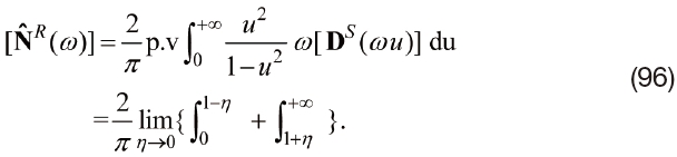
and the imaginary part

of its Fourier transform

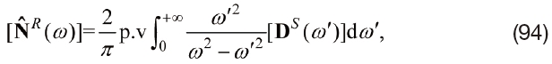
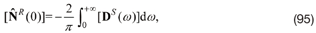
are related by the following relations that involve the Hilbert transform (see Ref. [22, 23]),
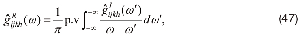
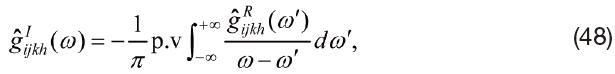
in which p.v denotes the Cauchy principal value which is defined as,

The relations defined by Eqs. (47) and (48) are also called as the Kramers and Kronig relations for the function
6. Boundary Value Problem in Terms of {u, p}
The boundary value problem in terms of {u,


In case of a free surface in the internal acoustic cavity (see Section 4.3), we must add the following boundary condition

We are interested in studying the linear vibrations of the coupled system that is around a static equilibrium and this is considered as a natural state at rest (then, the external solid and acoustic forces are assumed to be in equilibrium).
Eq. (50) corresponds to the structure equation (see Eqs. (17) and (28)), in which {divσ(u)}i = σij, j (u).
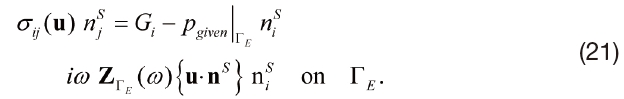
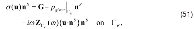
Eqs. (51) and (52) are the boundary conditions for the structure (see Eqs. (21) and (22)).
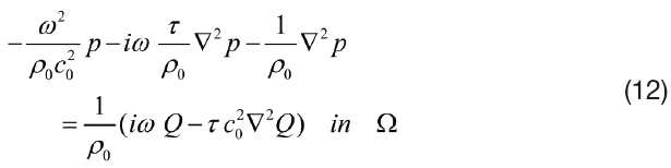
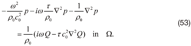
Eq. (53) corresponds to the internal dissipative acoustic fluid equation (see Eq. (12)).
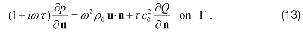
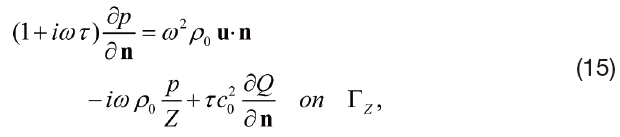
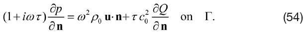
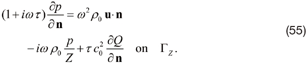
Finally, Eqs. (54) and (55) are the boundary conditions for the acoustic cavity (see Eqs. (13) and (15)).
It is important to note that the external acoustic pressure field pE has been eliminated as a function of u by using the acoustic impedance boundary operator ZΓE(ω) while the internal acoustic pressure field p is kept.
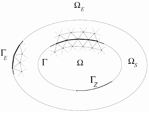
The computational model is constructed by using the finite element discretization of the boundary value problem. We also consider a finite element mesh of structure, Ω
We classically use the finite element method to construct the discretization of the variational formulation of the boundary value problem. This is defined by using Eqs. (50) to (55), with additional boundary condition that is defined by Eq. (56) in the case of a free surface for an internal liquid. For the details that concern with the practical construction of the finite element matrices, refer to Ref. [3]. Let,

be a complex vector of the

be the complex vectors of
in which the complex matrix

is defined by,
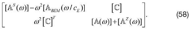
In Eq. (58), the symmetric (

is defined by,

where,
and

are symmetric (
is positive and invertible (positive definite). Matrices

and
are positive and not invertible (positive semidefinite). This is due to the presence of six rigid body motions since the structure has been considered as a free-free structure. The symmetric (

is defined by,

Where,
and
are symmetric (
is positive and invertible. Matrices

and
are positive and are not invertible with rank
in which τ(ω) is defined by Eq. (11). The internal fluid-structure coupling matrix
is related to the coupling between the structure and the internal fluid on an internal fluid-structure interface. This is a (
and
on the internal fluid-structure interface. The wall acoustic impedance matrix

is a symmetric (
on boundary Γ
which depends on ω/c
on the external fluid-structure interface Γ

in which [

is a sparse (
8. Reduced-Order Computational Model
The strategy used for the construction of the reduced-order computational model consists in using the projection basis constituted of [3]:
the undamped elastic structural modes of the structure in vacuo for which the constitutive equation corresponds to elastic materials (see Eq. (45)), and consequently, the stiffness matrix has to be taken for ω = 0.
the undamped acoustic modes of the acoustic cavity is with fixed boundary and without wall acoustic impedance. Two cases must be considered: one for which the internal pressure varies with the variation of the volume of the cavity (a cavity with a sealed wall is called as a closed cavity) and the other one for which the internal pressure does not vary along with the variation of the volume of the cavity (a cavity with a non sealed wall is called as an almost closed cavity).
8.1 Computation of the elastic structural modes
This step concerns with the finite element calculation of the undamped elastic structural modes of structure Ω

It can be shown that there is a zero eigenvalue with multiplicity 6 (corresponding to the six rigid body motions) and that there is an increasing sequence of

Let
be the eigenvectors (the elastic structural modes) that is associated with

Let 0 <
that is associated with the first

One has classical orthogonality properties,


where, [
(the eigenfrequencies are,
8.2 Computation of the acoustic modes
This step concerns the finite element calculation of the undamped acoustic modes of a closed (sealed wall) or an almost closed (non sealed wall) acoustic cavity, Ω. By setting λ = ω2, we then have the following classical (

It can be shown that there is a zero eigenvalue with multiplicity 1 and denoted as λ0 (corresponding to constant eigenvector denoted as

). Moreover, there is an increasing sequence of

Let
be the eigenvectors (the acoustic modes) that is associated with λ1, …, λα, …
Closed (sealed wall) acoustic cavity. Let be 0 < N ≤ n. We introduce the (n × N) real matrix of the constant eigenvector
and of the N ? 1 acoustic modes
that is associated with the first N ? 1 strictly positive eigenvalues as,

Almost closed (non sealed wall) acoustic cavity. Let be 0 < N ≤ n ? 1. We introduce the (n × N) real matrix of N acoustic modes
is associated with the first N strictly positive eigenvalues,

One has classical orthogonality properties,


where, [
8.3 Construction of the reduced-order computational model
The reduced-order computational model, of order


Complex vectors q
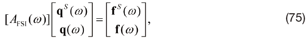
in which the complex matrix [
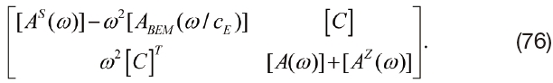
In Eq. (76), the symmetric (

in which [
and
The symmetric (

Where, [
Symmetric (
and finally, the symmetric (
The given forces are written as
and
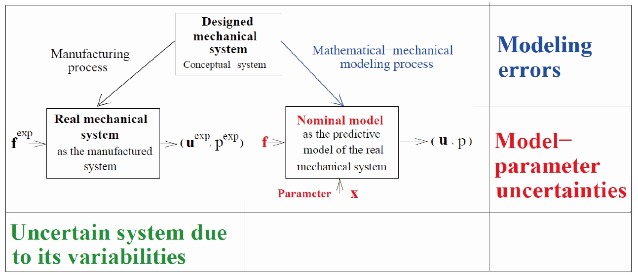
9.1 Short overview on uncertainty quantification
In this section, we summarize the fundamental concepts that are related to uncertainties and their stochastic modeling in computational structural-acoustic models (extracted from Refs. [33-34]).
9.1.1 Uncertainty and variability
The
there are
9.1.2 Types of approach for stochastic modeling of uncertainties
The
Concerning model uncertainties that is induced by modeling errors, it is well understood that the prior and posterior probability models of the uncertain parameters of the computational model are insufficient and they do not have the capability to take into account the model uncertainties in the context of computational mechanics as explained, for instance, in Ref. [41] and in Ref. [42-44]. Two main methods can be used to take into account the model uncertainties (modeling errors).
(i)
(ii)
to validate, using the experimental results, the nonparametric probabilistic approach of both the computational model-parameter uncertainties and the model uncertainties that are induced by modeling errors (Refs. [8, 44, 55-60]),
to extend the applicability of the theory to other areas (Refs. [61-69]),
to extend the theory to new ensembles of positive-definite random matrices that yield a more flexible description of the dispersion levels (Ref. [70]),
to apply the theory for the analysis of complex dynamical systems in the medium-frequency range that include structural-acoustic systems, (Refs. [8,33,55,57,59-61,71-76]),
to analyze nonlinear dynamical systems (i) with local nonlinear elements (Refs. [64, 77-83]) and (ii) with nonlinear geometrical effects (Refs. [84-85]).
Concerning the coupling of the parametric probabilistic approach of uncertain computational model parameters, with the nonparametric probabilistic approach of model uncertainties that are induced by modeling errors, a methodology has been recently proposed in Refs. 86-87. This generalized probabilistic approach of uncertainties in computational dynamics uses the random matrix theory. The proposed approach allows the prior probability model of each type of uncertainties (uncertainties on the computational model parameters and model uncertainties) which are to be separately constructed and identified.
Concerning robust updation or robust design optimization consists of updating a computational model or in optimizing the design of a mechanical system with a computational model by taking into account the uncertainties in the computational model parameters and the modeling uncertainties. An overview of the computational methods in optimization that considers uncertainties can be found in Ref. [88]. Robust updating and robust design developments with uncertainties in the computational model parameters are developed in Refs. [89-91] while robust updating and robust design optimization with modeling uncertainties can be found in Refs. [82, 92-95].
9.2 Uncertainties and stochastic reduced-order computational structural-acoustic model
This section is devoted to the construction of the stochastic model of both computational model- parameters uncertainties and modeling errors by using the nonparametric probabilistic approach and random matrix theory (for the details, see Refs. [33-34, 49, 59]). We apply this methodology to the reduced-order computational structural acoustic model that is defined by using Eqs. (73) to (78). It is assumed that there is no uncertainties in the boundary element matrix [A


Where, for all fixed ω, the complex random vectors Q
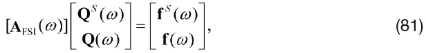
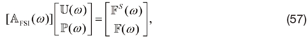
Where, the complex random matrix [AFSI(ω)] is written as,
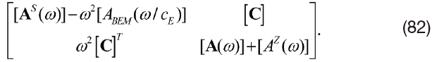
The symmetric (

Where, the positive-definite symmetric (

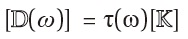
Where, [M], [D(ω)] and [K]are symmetric (

in which τ(ω) is deterministic and it is defined by Eq. (11). For a closed (sealed wall) acoustic cavity, random matrix
[K] is positive and it is not invertible with rank
In the framework of the nonparametric probabilistic approach of uncertainties the probability distributions and the generators of independent realizations of such random matrices. They are constructed by using random matrix theory [48] and the maximum entropy principle [51, 67] from Information Theory [52], in which Shannon introduced the notion of entropy as a measure of the level of uncertainties for a probability distribution. For instance, if
The maximum entropy principle consists in maximizing the entropy, that is to say, maximizing the uncertainties, under the constraints that are defined by the available information. Consequently, it is important to define the algebraic properties of the random matrices for which the probability distributions are to be constructed. Let
Consequently, we have
It is well known that a real Gaussian random variable can take in negative values. Consequently, the Gaussian orthogonal ensemble (GOE) of random matrices [48] is the generalization for the matrix case of the Gaussian random variable which cannot be used when the positiveness property of the random matrix is required. Therefore, new ensembles of random matrices are required for the implementation of the nonparametric probabilistic approach of uncertainties. Below, we summarize the construction [42-43] of an ensemble of positive-definite symmetric (
9.3.1 Definition of the available information
For the probabilistic construction using the maximum entropy principle, the available information corresponds to two constraints. First is the mean value which is given and it is equal to the identity matrix. Second is an integrability condition which has to be imposed in order to ensure the decrease in the probability density function around the origin. These two constraints are written as,

Where, [
9.3.2 Probability density function
The value of the probability density function of the random matrix [G0] for the matrix [

and the integration is carried out on the set of all the positive-definite symmetric (

is,
Let δ be a positive real number defined by,
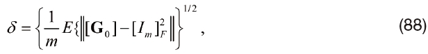
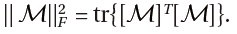
and this will allow the dispersion of the probability model of the random matrix [G0] that is to be controlled and ∥
For δ such that 0 < δ < (m+1)1/2(m+5)?1/2, the use of the maximum entropy principle under the two constraints are defined by using Eq. (86) and the normalization condition is defined by Eq. (87). This yields, for all positive-definite symmetric (

Where, the positive constant of normalization is
9.3.3 Generator of independent realizations
The generator of the independent realizations (which is required to solve the random equations with the Monte Carlo method) is constructed by using the following algebraic representations. By using the Cholesky decomposition, random matrix [G0] is written as [G0] = [L]
random variables {[L]ij´, j ≤ j´} are independent;
for j < j´, the real-valued random variable [L]jj´ is written as, [L]jj´ = σmUjj´ where, σm = δ(m+1)?1/2 and Ujj´ is a real-valued Gaussian random variable with zero mean and variance equal to 1;
for j = j´, the positive-value random variable [L]jj is written as,
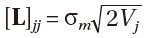
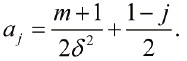
in which Vj is a positive-valued Gamma random variable with probability density function Γ(aj, 1)
where,
9.3.4 Ensemble SG+ε of random matrices
Let 0 ≤ ε << 1 be a positive number (for instance, ε can be chosen as 10?6). We then define the ensemble

of all the random matrices such that
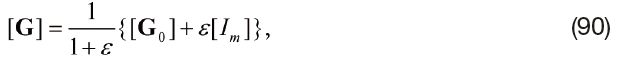
Where, [G0] is a random matrix whose probability density function is defined in Section 9.3.2 and whose generator of independent realizations is defined in Section 9.3.3.
9.3.5 Cases of several random matrices
It can be proved (Ref. [44]) that if there are several random matrices for which there is no available information concerning their statistical dependencies then, the use of the maximum entropy principle yields the best model that maximizes the entropy (the uncertainties). This is a stochastic model for which all these random matrices are independent.
9.4 Stochastic modeling of random matrix [MS]
As there is no available information that concerns to the statistical dependency of [M

Where, [G
which is defined in Section 9.3.4. Its probability distribution and generator of independent realizations depend only on the dimension
9.5 Stochastic modeling of the family of random matrices [DS(ω)] and [KS(ω)]
As there is no available information concerning the statistical dependency of the random matrices {[D


For ω ≥ 0, the construction of the stochastic model of the family of random matrices [D
Constructing the family [DS(ω)] of random matrices such that [DS(ω)] = [LDS(ω)]T[GDS][LDS(ω)] where, [LDS(ω)] is such that [DS(ω)] = [LDS(ω)]T[LDS(ω)] and where, [GDS] is a (NS × NS) random matrix that belongs to ensemble
and it is defined in Section 9.3.4. Its probability distribution and its generator of independent realizations depend only on the dimension NS and on the dispersion parameter δDS which allows the level of uncertainties to be controlled.
Defining the family

of random matrices such that
Constructing the family

of random matrices by using the equation,
or equivalently by using the two following equations that are useful for computation:
and, for ω > 0,
Defining the family

of random matrices such that
Constructing the random matrix [KS(0)] = [LKS(0)]T[GKS(0)] [LKS(0)] where, [LKS(0)] is such that [KS(0)] = [LKS(0)]T[LKS(0)] and where [GKS(0)] is a (NS × NS) random matrix that belongs to ensemble
is defined in Section 9.3.4. Its probability distribution and generator of independent realizations depend only on the dimension NS and on the dispersion parameter δKS(0) which allows the level of uncertainties to be controlled. It should be noted that the random matrix [GKS (0)] is independent of random matrix [GDS].
Computing the random matrix
Defining the random matrix
Constructing the random matrix
and verifying that [KS(ω)] is an effectively increasing function on [0, +∞[.
9.6 Stochastic modeling of random matrix [M]
As there is no available information concerning the
statistical dependency of [M] with the other random matrices of the problem, the random matrix [M] is independent of all the other random matrices. The deterministic matrix [

Where, [G
and it is defined in Section 9.3.4. Its probability distribution and generator of independent realizations depend only on the dimension
9.7 Stochastic modeling of random matrix [K]
As there is no available information concerning the
statistical dependency of [K] with the other random matrices of the problem, the random matrix [K]is independent of all the other random matrices. For the stochastic modeling of [K], two cases have to be considered.
Closed (sealed wall) acoustic cavity. In such a case, the symmetric positive matrix [K] is of rank N ? 1 and it can then be written as [K] = [LK]T [LK] where, [LK] is a rectangular (N, N ? 1) real matrix. By using the nonparametric probabilistic approach of uncertainties, the stochastic model of the positive symmetric random matrix [K] of rank N ? 1 is then defined [44] by,

Where, [G
and it is defined in Section 9.3.4. It’s probability distribution and generator of independent realizations depend only on the dimension
Almost closed (non sealed wall) acoustic cavity.
The matrix [

Where, [G
and it is defined in Section 9.3. It’s probability distribution and generator of independent realizations depend only on the dimension
9.8 Stochastic modeling of random matrix [C]
As there is no available information concerning the statistical dependency of [C] with the other random matrices of the problem, the random matrix [C] is independent of all the other random matrices. We use the construction that is proposed in Ref. [44]) in the context of the nonparametric probabilistic approach. Let us assume that

Where, [G
and it is defined in Section 9.3.4. It’s probability distribution and generator of independent realizations depend only on the dimension
9.9 Comments about the stochastic model parameters of uncertainties and the stochastic solver
The dispersion parameter δ of each random matrix [G] allows its level of dispersion (statistical fluctuations) to be controlled. The dispersion parameters of random matrices [G

This belongs to an admissible set
For a given value of δ, there are two major classes of methods for solving the stochastic reduced-order computational structural-acoustic model and it is defined by using Eqs. (79) to (85). The first one belongs to the category of the spectral stochastic methods (see Refs. [35-36,97]). The second one belongs to the class of stochastic sampling techniques for which the Monte Carlo method is the most popular. Such a method is often called non-intrusive as it offers the advantage of only requiring the availability of classical deterministic codes. It should be noted that the Monte Carlo numerical simulation method (see for instance Refs. [98-99]) is a very effective and efficient method as it as the four following advantages,
it is a non-intrusive method,
it is adapted to massively parallel computation without any software developments,
it is such that its convergence can be controlled during the computation,
the speed of convergence is independent on the dimension.
If the experimental data are available then, there are several possible methodologies (whose one is the maximum likelihood method) to identify the optimal values of δ (for the sake of brevity, these aspects are not considered in this paper and we refer the reader to Ref. [33]).
10. Symmetric Boundary Element Method Without Spurious Frequencies for the External Acoustic Fluid
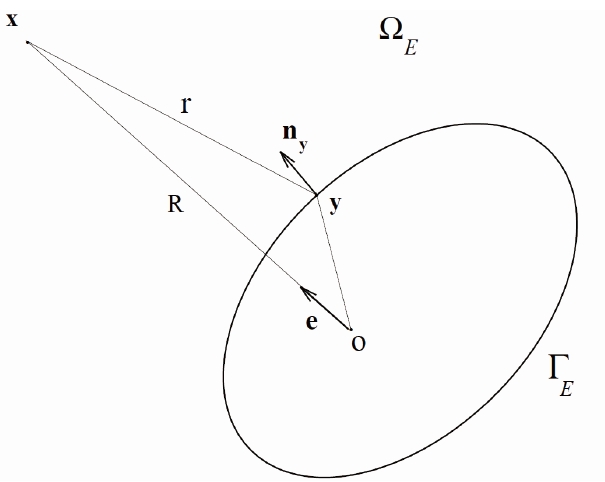
The inviscid acoustic fluid occupies the infinite three-dimensional domain Ω
Many methods can be found in literature for solving this problem: the boundary element methods, the artificial boundary conditions and the local/nonlocal non-reflecting boundary condition (NRBC) to take into account the Sommerfeld radiation condition at infinity, the Dirichlet-to-Neumann (DtN) boundary condition are related to a nonlocal artificial boundary condition and they match the analytical and numerical solutions, the infinite element method, the doubly asymptotic approximation method, the finite element method in unbounded domain and related a
The frequency-dependent impedance boundary operator ZΓ
The finite element discretization of the boundary integral equations yields the Boundary Element Method [3, 118-121]. Furthermore, most of those formulations yield unsymmetric fully populated complex matrices. The computational cost can then be reduced by using fast multipole methods [122-126].
A major drawback of the classical boundary integral formulations for the exterior Neumann problem related to the Helmholtz equation. This is related to the uniqueness problem although the boundary value problem has a unique solution for all real frequencies [18, 127]. Precisely, there is no unique solution of the physical problem for a sequence of real frequencies called as
In this section, we present a method that was initially developed in Ref. [134]. This yields an appropriate symmetric boundary element method that is valid for all real values of the frequency and it is numerically stable and very efficient. This method is detailed in Ref. [3]. It does not require introduction of additional degrees of freedom in the numerical discretization for the treatment of irregular frequencies. This method has been extended to the Maxwell equations [138]. In the case of an external liquid domain with a zero-pressure free surface (which is not presented here for the sake of brevity) the method presented below can be adapted by using the image method (for the details, see Ref. [3]).
10.1 Exterior Neumann problem related to the Helmholtz equation
The geometry is defined in Fig. 5. The inviscid fluid occupies the infinite domain Ω

Where, ρ


with
10.2 Pressure field in ΩE and on ΓE
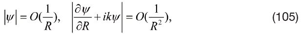
For arbitrary real ω ≠ 0, it can be shown that the boundary value problem is defined by using Eqs. (103) to (105). It admits a unique solution that is denoted by ψsol. It depends linearly on the normal velocity

be the value of ψsol on Γ

We also introduce the linear boundary operator BΓ

By using Eq. (102), for all x in Ω

in which Z

Similarly, the pressure field

where, ZΓ

Note that ZΓ
10.3 Symmetry property of the acoustic impedance boundary operator
The transpose of the operator BΓ

and from Eq. (111), we deduce that

It should be noted that these complex operators are symmetric but not hermitian.
10.4 Positivity of the real part of the acoustic impedance boundary operator
Operator

Where, MΓ


It can be shown that (Ref. [3]) the following positivity property of the real part DΓ
10.5 Construction of the acoustic impedance boundary operator for all real values of the frequency
We present here an appropriate symmetric boundary element method without spurious frequencies, for which the details can be found in Ref. [3]. This formulation simultaneously uses two boundary singular integral equations on Γ
The linear boundary integral operators S
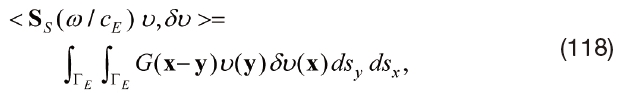
Where,

Where,

It can be proven that the operator H(ω/c
This classical boundary equation that allows the velocity potential to be calculated for a given normal velocity, has a unique solution for all real ω . It does not belong to the set of frequencies for which S
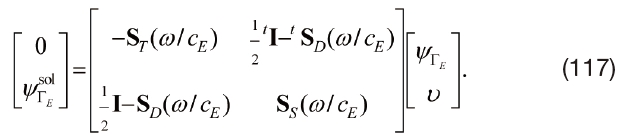
This yields the solution
for all real ω as the elements that belong to the null space are filtered when ω is a spurious frequency. Concerning the practical construction of
for all real values of ω, by using Eq. (117), a particular elimination procedure will be described in Section 10.7.
10.6 Construction of the radiation impedance operator
The solution {ψsol (x, ω), x ∈ Ω
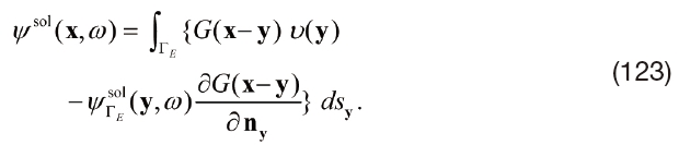
For all x that is fixed in Ω

By using Eq. (107), Eq. (123) can be rewritten as
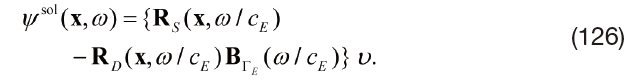
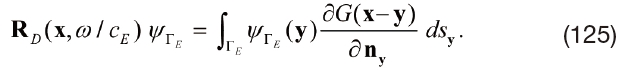
From Eq. (106), we deduce that for all x fixed in Ω
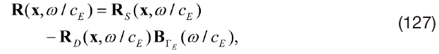
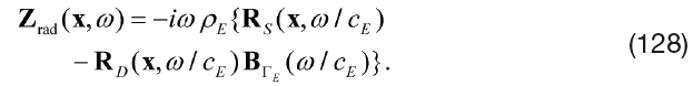
and the radiation impedance operator Zrad(x, ω) is calculated by using Eqs. (109) and (127),
10.7 Symmetric boundary element method without spurious frequencies
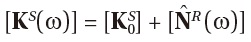
We use the finite element method to discretize the boundary integral operators S

Where, the symmetric complex matrix [
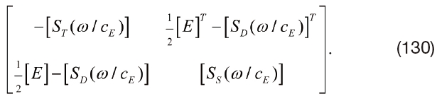
In Eq. (129),

is the complex vector of the nodal unknowns that correspond to the finite element discretization of

The matrix [
and V that defines the symmetric (

The particular elimination procedure discussed in Section 10.5 which avoids the spurious frequencies is defined below. Vector ΨΓ

of dimension

Finally, the finite element discretization of the acoustic radiation impedance operator Zrad(x, ω) defined by Eq. (129) is written as,

10.8. Acoustic response to prescribed wall displacement field and acoustic source density
We now consider the acoustic response of the infinite external acoustic fluid submitted to a prescribed external acoustic excitation, namely an acoustic source
Pressure in Ω

where,

The pressure
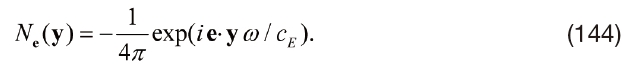
where,
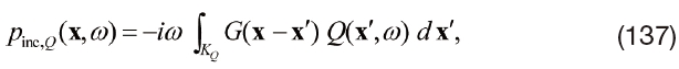
where, the Green function
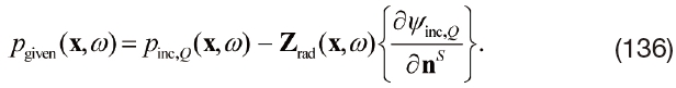
Pressure on Γ

where,

and the pressure field
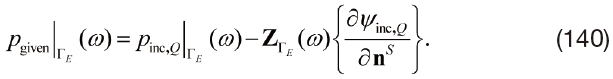
By substituting Eq. (139) in (138), it yields

For details, we refer the reader to Chapter 12 of Ref. [3] .
10.9 Asymptotic formula for the radiated pressure farfield
At point x in the external domain Ω

Definition of integral operators
and
For all x =
Ω
and
by,
Where,
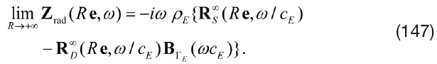
Asymptotic formula for radiation impedance operator Z


From Eq. (127), we deduce the asymptotic formula for theradiation impedance operator as,
We have presented an advanced computational formulation for dissipative structural-acoustics systems and fluid-structure interaction. This is adapted for the development of a new generation of software. An efficient stochastic reduced-order model in the frequency domain is proposed to analyze low- and medium-frequency ranges. All the required modeling aspects for the analysis of the mediumfrequency domain have been introduced namely, a viscoelastic behavior for the structure, an appropriate dissipative model for the internal acoustic fluid which includes wall acoustic impedance and a model of uncertainty in particular for modeling errors.