Supersonic base flows are characterized by several complex turbulent flow features as benchmark test problems in the aerodynamic drag prediction [1,2]. These flows are characterized by separating boundary layers that interact with the recirculating flow leading to a recompression region and a wake region [3]. Accurate prediction of such flow features requires advanced turbulence models, which include both the compressibility effects [4-5] and the non-equilibrium effects of turbulence [6]. For two-equation turbulence models, improvements in predictions have been achieved by reducing the production of the turbulent kinetic energy, or by increasing the dissipation rate of kinetic energy.

One of the important requirements for good turbulence models is the realizability condition that is not usually satisfied directly in any linear eddy-viscosity formulation [7]. Several researchers [8-12] have found that the realizability constraints could be fulfilled by decreasing the eddy viscosity, and that nonlinear eddy viscosity models or weakly nonlinear eddy viscosity formulations improve the performance of the turbulence models for flows in the presence of adverse pressure gradients, particularly involving shock wave/boundary-layer interactions. The realizability condition has been considered in several ways. For the k-ω SST model [11,12], the eddy viscosity formulation was derived based on the results of Bradshaw et al.[7] in the adverse pressure gradient regions. Coakley [8] and Durbin [9] proposed fundamentally identical corrections. The essential points regarding these corrections are to reduce the magnitude of the eddy viscosity and to produce an asymptotic behavior of the eddy viscosity coefficient when the mean strain rate leans toward infinity.

Several successful implementations of k-ε turbulence models [13-16] have also been made by reducing the eddy viscosity. A nonlinear eddy viscosity model of Craft et al.[15] used an eddy viscosity coefficient that is a function of the strain rate or the magnitude of vorticity and turbulent Reynolds number. Though the eddy viscosity function results in a reduction of the magnitude for the eddy viscosity when the mean strain rate is large, the function is essentially chosen to model the near-wall effects and to optimize the coefficients based on experimental data or Direct Numerical Simulations (DNS). Barakos and Drikakis [16] argued that the success of the cubic non-linear eddy viscosity is based on the functional coefficient used, not on the non-linear cubic expansion of the shear stresses. Therefore, an improved formulation for the k-ε turbulence model is likely to be achieved with the proper implementation of the realizability condition, rather than in the development of complex higher order constitutive relations.

In addition to turbulence modeling, spatial discretization schemes play an important role for the accurate prediction of base flows, since regions of high pressure and density gradients over a wide range of Mach numbers exist. The previous work [11] for the transonic flow past airfoils showed that the velocity profiles obtained from the second-order accurate spatial discretization of the turbulence variables are more accurate than the results obtained from the first-order accurate discretization of the turbulence equations. From the numerical experiments, the difference in the results obtained with schemes of different spatial accuracy was observed to be comparable to the differences in the results obtained with variants of the k-ε turbulence models.

In the present paper, several turbulence models have been examined. They include the variants of the Launder-Sharma k-ε model [13,14] adopting the eddy viscosity formulation of Craft et al.[15]. The performance of these various models was examined for supersonic base flows. The compressibility modifications [3-6] for the k-ε turbulence models were also investigated. Based on the results obtained, a simple modification based on the realizability principle is proposed to the Launder-Sharma model, and the prediction capability of the improved model was demonstrated.

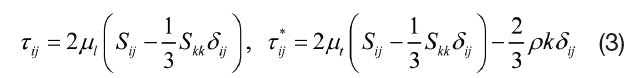
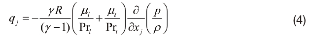
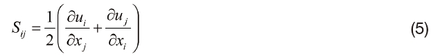
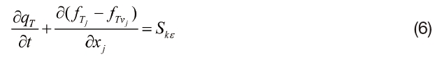
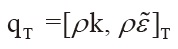
In the present work, the compressible Navier-Stokes equations and the k-ε turbulence equations were considered. The Navier-Stokes equations are

where q is the flow variable vector, and fj and fvj are the inviscid and viscous fluxes in each direction,

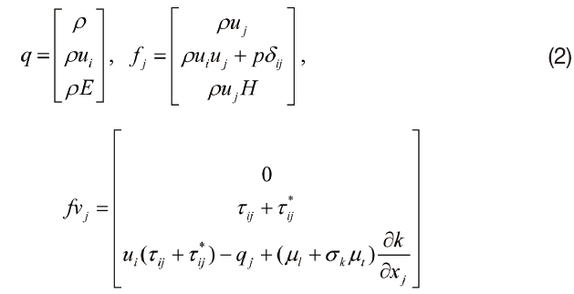
Here ρ and p are the density and pressure, u_i are the Cartesian velocity components, E is the total energy, and H = E + p/ρ is the total enthalpy. The quantity τ_ij and τ*_ij are the laminar and turbulent stresses, respectively, and qj represents the total heat flux in each direction. These quantities are defined as:

where γ is the ratio of specific heats and R is the gas constant. The variables Pr_l and Pr_t are the laminar and turbulent Prandtl numbers, respectively. The quantity μ_l is the molecular viscosity determined by the Sutherland law and μ_t is the eddy viscosity, based on the turbulence model used, which is defined later. The term S_ij is the velocity strain rate tensor defined as:

2.1.1. The Launder-Sharma k-ε model [13,14]

In the k-ε turbulence model as originally proposed by Launder and Sharma, the turbulence equations can be written as

where

and the convection and diffusion terms of the turbulence equations are expressed as

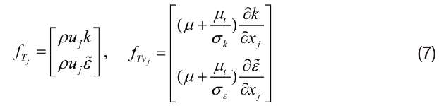
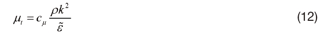
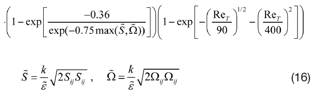
where S is the mean strain rate and the eddy viscosity is written in terms of k and

as

In the Launder-Sharma model, the eddy viscosity function is written as

where

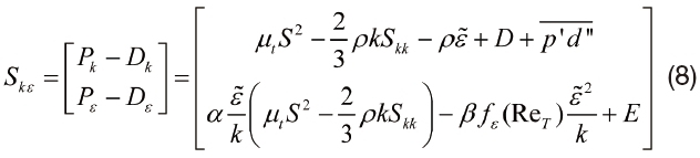
In the above equations, ReT is the turbulence Reynolds number and the term D and E model the near-wall effects. The pressure-dilatation term

will be described later. The term D models the ‘anisotropic part’ of the dissipation rate where

is the ‘isotropic’ dissipation rate:

The low-Reynolds term E is expressed as

The closure constants of the Launder-Sharma model are σ_k=1.0, σ_ε=1.3, α=1.44, β=1.92. The damping function f_ε is defined by

In this paper, the term c_μ is defined to include the Reynolds number-dependent damping term (f_μ shown in [14]). The details concerning the preceding turbulence closure may be found in the original references [13-15].

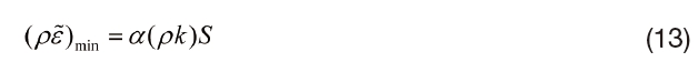
In order to stabilize the computation and prevent excessive turbulent kinetic energy, we impose a direct limiter on the Launder-Sharma model as

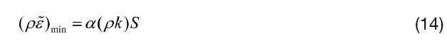
This realizability-like limiter is applied at every iteration step as in [11] and has an effect similar to the realizability condition.

2.1.2 A linear version of the k-ε Craft model [15,16]

Craft et al.[15] devised a non-linear eddy viscosity model, which employed a suitable cubic stress-strain relation (not shown here) and a function cμ based on the strain and vorticity invariants:

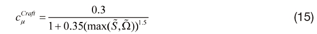
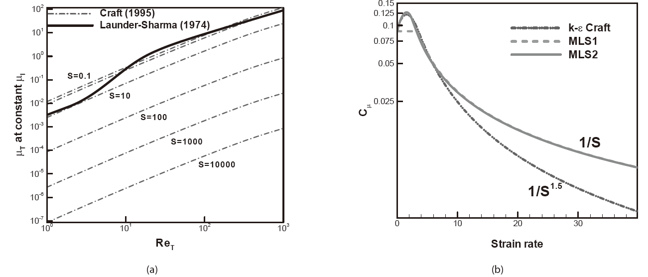
The function cμ was optimized so that the predicted variation of the Reynolds stresses with strain rate is in good agreement with both experimental and direct numerical simulation data from a homogeneous shear flow. In the present linear version, Eq. (15) is used in the eddy viscosity expression but with a linear stress-strain relationship in Eq. (16). Craft et al. also modified the term E in order to reduce its dependence on the Reynolds number at low turbulent Reynolds numbers, but this modification is not used in the present implementation for simplicity.

2.1.3 A modified Launder-Sharma (LS) model

The k-ω models were tested for un-separated and separated transonic flows to examine the effect of the weakly non-linear eddy viscosity model of Wilcox and Durbin (WD+ model) [10,11]. Numerical results showed that the WD+ model using the weakly nonlinear eddy viscosity exhibited better overall performance compared to the linear Wilcox model [17] and the SST model. Our numerical experiments show that the realizability condition improves the accuracy of predictions as well as enhances the robustness by preventing unphysical turbulent kinetic energy for transonic and supersonic flows. As shown by Gerolymos [14], in order to stabilize the computations, k and ε should be bounded by positive cutoff values. The k-ε computations often begin from a previous computation using a robust turbulence model in order to achieve an initial flow field. These approaches are problem-dependent or sometimes impractical with regards to complex geometries. The instability in the initial phase of computations can be successfully prevented by applying the realizability condition to k-ε turbulence models. Therefore, we can improve the Launder-Sharma model by incorporating a dependence on the mean strain rate within the variation of the c_μ function. This is equivalent to adding a realizability constraint to the Launder-Sharma k-ε model. Therefore, the following realizability condition is applied to the Launder-Sharma k-ε model:

Equation (17) dramatically improves the robustness of the Launder-Sharma model without the need for applying direct limiters, such as Eq. (14), to turbulence quantities. Equation (17) can be viewed as another form of the realizability constraint: it accepts the Launder-Sharma eddy viscosity so long as it is well-behaved, but limits it with a realizability model once the eddy viscosity exceeds some bounds. This will be referred to as the modified LS (MLS1) model.

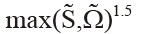
Barakos and Drikakis [16] examined the performance of the cubic non-linear eddy viscosity models and found them to be superior to the linear models based on the linear stress-strain relations. They argued that the success of the Craft et al. model [15] comes from the functional cμ expression utilized, and not from the non-linear cubic expansion of the shear stresses. Based on their arguments, it would be worthwhile to use a functional c_μ in conjunction with a linear two-equation model. To investigate the effect of the functional c_μ, the variation of the eddy viscosity with the turbulent Reynolds number is displayed in Fig. 1(a) at different strain rates, and shows that for the Craft model (Eq. (15)) the eddy viscosity is reduced with the strain rate S. This implies that the c_μ functional in the Craft model acts like the realizability condition, though it is not directly derived based on realizability considerations. Figure 1(b) shows that at higher strain rates the resulting c_μ in Eq. (15) is actually smaller than that in Eq. (17) based on the realizability condition. Indeed, for this reason, the Craft model is fairly robust and behaves better than other well-known variants of the k-ε models. It should be noted that c_μ of the Craft model,

which was optimized from the DNS and numerical data, exceeded 0.09 at the region of small strain rates. The present numerical experiments show that this aspect provides good velocity distributions in the recirculating region.

The obvious difference between the expression proposed here and that proposed by Craft et al. is that Eq. (15) is inversely proportional to the

and Eq. (17) is inversely proportional to

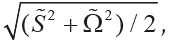
respectively. This difference might cause a different behavior in the TKE production term in each model. We follow the analysis noted by Thivet et al.[18] in order to explore potential improvements in regards to the realizability constraint. When crossing a shock wave normal to the x direction, the strain rate behaves like:

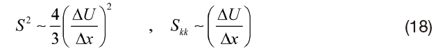
The production Pk, which, summed up over the cell volumes, can be written as:

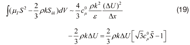
We can easily find the production term of the k-ε model behaves as 1/Δx in the cell crossed by the shock wave, when Δx goes towards zero, and if c_μ is held constant. This behavior may cause grid dependence and result in excessive turbulence production for some situations. This dependence can be eliminated by imposing a cμ function based on the realizability condition, such as Eq. (15) or Eq. (17). Then, for a large mean strain rate, the production terms are

The results show that the production rate of the linear Craft model is proportional to √Δx for a large mean strain rate and that the rate of the modified Launder-Sharma model proposed here is independent of mesh size. This also implies that unlike the modified LS Model, the TKE production of the linear Craft model could be unphysical since it does not guarantee a positive value of the TKE production when the flow crosses a shock wave. From this, we attempt to modify the function of Eq. (15) so that the production rate is independent of the mesh size. This modified expression termed as the MLS2 model here is given by:

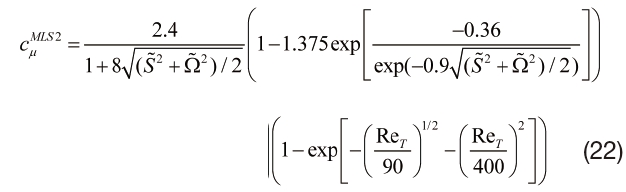
As shown in Fig. 1(b), the resulting formulation, Eq. (22), follows the variation of the Craft model at low non-dimensional strain rates and the realizability bound at high strain rates.

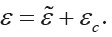
In order to account for the compressibility effects, the models of Sarkar [4], Wilcox [5] and Ristorcelli [6] are considered; they account for the dilatational dissipation, which represents the added rate of dissipation regarding turbulent kinetic energy. The dissipation rate ε in the k equation can be split into a solenoidal part and a dilatational part, c, which is defined by the compressibility modification used:

2.2.1 Sarkar model

where M_t = √2k / a is the turbulent Mach number and a is the speed of sound. The pressure dilatation term (Eq. (8)) is modeled as

2.2.2 Wilcox model

Here, the compressibility term is modeled as:

where H is the heaviside step function.

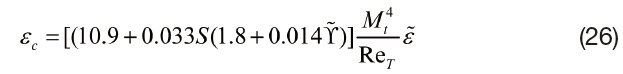
2.2.3 Ristorcelli model

Ristorcelli [6] proposed a compressibility modification for dilatational dissipation and pressure dilatation through statistical data and theory. Though his model has a number of heuristic constants and complex terms (not shown in this paper), it is shown to distinguish the characteristics of the compressible free shear layer from that of the boundary layer. Here, a simplified model is used, which has the leading terms of the original Ristorcelli model:

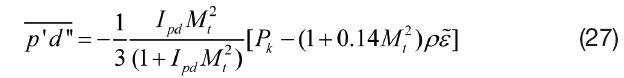
where

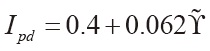
and

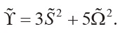
As shown in Eq. (26) and Eq. (27), the dilatational dissipation is very small

compared to the other compressibility modifications and the pressure-dilatation term is dominant when the flow is in a non-equilibrium state.

The governing equations in the physical coordinate system were transformed into computational body-fitted coordinates and were discretized by a cell-centered finite volume method. The HLLE+ [19] and the third-order MUSCL schemes [20] were used with the minmod limiter to obtain second-order spatial accuracy. Central differencing was applied to obtain variable gradients of the viscous flux. As discussed in [11], a second-order scheme for the turbulence variables produces more accurate flow predictions compared to those from a first-order scheme for separated flows. To enhance the robustness for supersonic flows, the same MUSCL second-order scheme, which was used for the Navier-Stokes solver, was also employed for the turbulence variables.

The diagonalized alternating-direction implicit (DADI) method was used as the solver to determine the steady-state solutions [11]. It should be noted that the contribution of the viscous terms cannot be simultaneously diagonalized, in contrast to the inviscid terms, and it was added in the implicit part only through an approximation of spectral radius scaling. An algorithm was used to integrate the Navier-Stokes and the turbulence equations sequentially. In the present implicit algorithm, the turbulence equations were iterated only once per time step because more iterations do not reduce the total computing time for the implicit method. The source vectors for each turbulence model were treated implicitly, because otherwise, it would have resulted in a stiffness problem in the time-marching methods. The contributions of the turbulent dissipation terms were added in the implicit parts to increase the diagonal dominance, whereas the production contributions were treated explicitly. Additional details regarding the numerical scheme used to solve the Navier-Stokes and the turbulence equations can be found in [11] and the source term linearization method is well documented in [21].

Boundary conditions affect the accuracy as well as the

convergence of the numerical scheme. At the solid walls, no-slip conditions for velocities were applied and the density and energy were extrapolated from the interior cells. The value of k and

was set to zero at the wall for the present k-ε turbulence models.

To examine the performance of the turbulence models, a turbulent supersonic flow[1-3] past an axisymmetric base was studied. The freestream conditions were M_∞ = 2.46 and R_e = 5.2×10⁷/m based on the freestream velocity and the base diameter. A schematic of this flow is shown in fig. 2. Detailed experimental data for this flow condition and geometry are available [1]. The inflow velocity distribution was prescribed and obtained from EDDYBL code of Wilcox’s [22].

Results were obtained with the four 2-equation turbulence models discussed earlier: (1) the Launder-Sharma k-ε model (LS) with the direct limiter, Eq. (14), (2) the Craft model which denotes the Launder-Sharma model with c_μ formulation of Craft et al., Eq. (15), (3) the present modified Launder-Sharma (MLS1) model with the realizability condition, Eq. (17), and (4) the MLS2 model with a new functional expression, Eq. (22), which combines the realizability constraint with the Craft formulation. Representative results from these 4 different turbulence models were compared with experimental data and presented in this section.

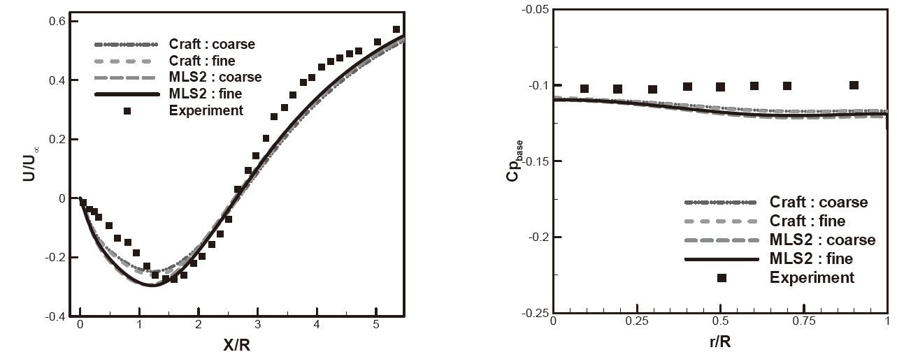
The computational grid consists of two blocks with 33×65 and 321×213 node points in each block. The smaller block was upstream of the step while the larger block was downstream. For grid independence, a coarse grid that was made of 21×51 and 201×150 node points was also used. The grids were stretched toward the wall in order to resolve the laminar viscous sub-layer. Centerline velocity and radial pressure profiles at the wall for the coarse and fine grids are shown in Fig. 3, respectively. Results were shown for two turbulence models (the Craft model and MLS2). The centerline velocity and radial wall pressure results on the two grids were nearly identical. The fine grid results were therefore expected to be grid independent. Unless otherwise stated, results were presented from the fine grid.

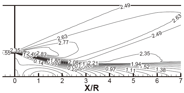
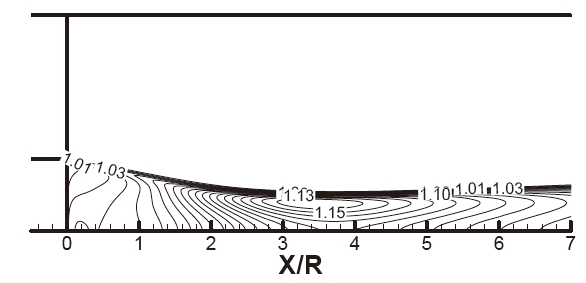
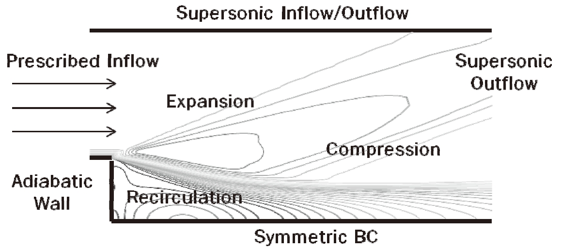
Figures 4 and 5 display field contours of Mach number and compressibility factor, (1+M²_t ), for the MLS2 model. The free shear layer separates the supersonic region from

the recirculating region. The Mach number contour shows an expansion at the corner and recompression of the main stream. Sharp velocity gradients of the free shear layer cause the production of turbulent kinetic energy (TKE). The maximum value of the turbulent Mach number (M_t) is approximately 0.4 at the X/R = 3.4 and the distribution implies that the compressibility modification cannot be ignored.

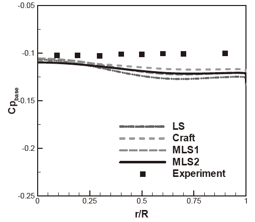
Figure 6 shows the pressure distributions along the base for different turbulence models. The base pressures predicted by the k-ε models are compared with the experimental data [1,3], which are relatively constant with respect to the radial distance. The base pressure predicted by the LS model shows a relatively larger variation in magnitude along the base, in contrast to the near-constant experimental data. The result using the MLS2 model shows a smaller variation in the base pressure, though the values were lower than those of the experimental data. The Craft model exhibits the closest agreement with experimental data compared to the other models.

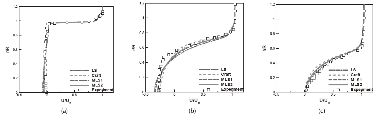
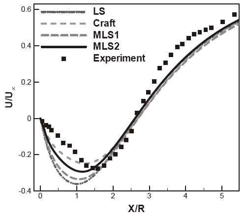
The streamwise velocity distributions along the centerline

are shown in Fig. 7 for the various turbulence models, and demonstrate the advantages of the present formulation. The Craft model gives better agreement with the experimental data compared to the other k-ε models. It is interesting to note that c_μ of the Craft and MLS2 models exceeded 0.09 at small strain rates and produced larger eddy viscosity in the recirculating region of this flow than those from the LS and MLS1 models. This increase in the eddy viscosity resulted in an increase in turbulent mixing and the reduction of the reverse velocity in the recirculation region.

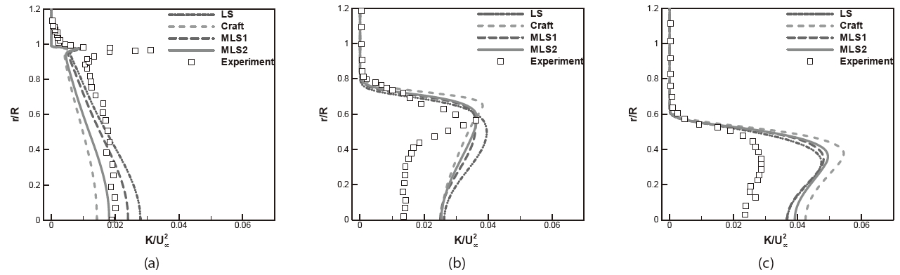
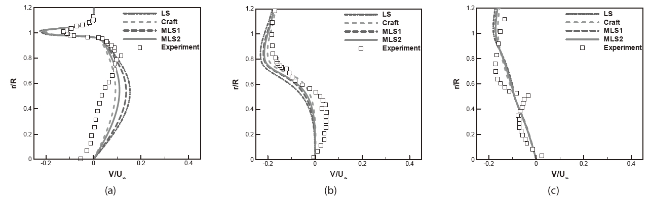
Figures 8 and 9 display U and V velocity profiles at specified streamwise locations. The turbulent kinetic energy profiles are compared in Fig. 10. The k-ε Craft model and the MLS2 model predictions of the velocity profiles are

in best agreement with the data. As shown in Fig. 10, the Craft model produced smaller TKE than the other models at X/R = 0.079 and 1.26. This is related to the definition of cμ, which is proportional to the inverse of

The only difference between the k-ε Craft model and the MLS2 model is the definition of the strain-related damping

coefficients in c_μ which causes the observed differences in the TKE distributions. It should be noted that the MLS2 model makes an improvement in the prediction of the TKE profiles. This indicates that it can be considered as an improvement of the k-ε Launder-Sharma model. However, there are still differences with the experimental data and room for improvements in the model.

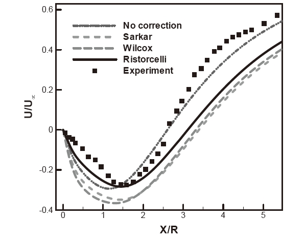
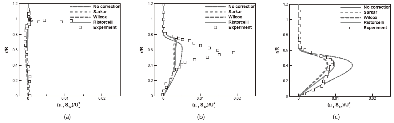
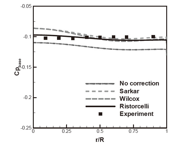
Streamwise velocity distribution along the centerline is displayed in Fig. 11 for the MLS2 model with compressibility modification. The Sarkar and the Wilcox compressibility modifications produce longer reattachment length and larger peak reverse velocity. These models introduce additional amounts of the TKE dissipation in the k equations, which is proportional to the square of the turbulent Mach number. The addition of the dissipation results in the reduction of the turbulent mixing and the increase in the reverse velocity. The simplified Ristorcelli model gives more accurate velocity distribution in the recirculating region and shows that the Ristorcelli model is superior to the other models with regards to the present non-equilibrium flow. The advantage of the Ristorcelli model is also shown in Fig. 12 for the wall pressure distribution. All modifications increase the pressure coefficient. The Sarkar and Wilcox models produce somewhat larger variations of the pressure distribution than the Ristorcelli model. The mean magnitude of the wall pressure of the Ristorcelli is in excellent agreement with the experimental data.

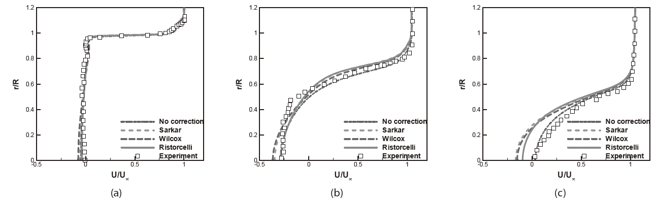
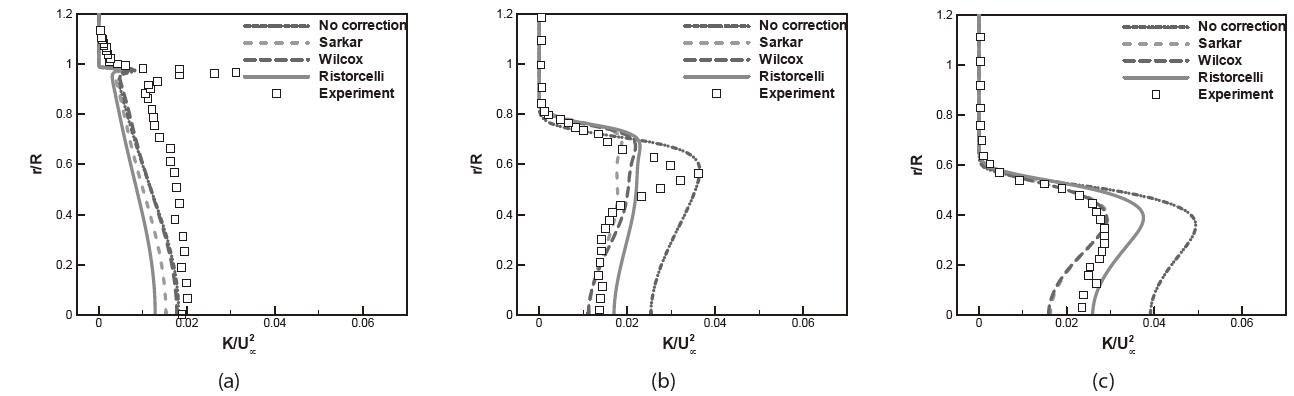
Velocity profiles, TKE, and primary Reynolds stress profiles with compressibility modification are examined in Figs. 13-15 for the MLS2 model. A more noticeable effect of these corrections can be observed in the TKE and the primary Reynolds stress profiles. As discussed earlier, the compressibility modification decreases the production of TKE and the Reynolds stress, particularly at X/R = 2.67. The Sarkar and Wilcox models give better TKE profiles than the Ristorcelli, whereas the velocity and the primary Reynolds stress distributions of the Ristorcelli model are in best agreement with the experimental data.

The performance of the k-ε models was examined for

supersonic base flow and two types of modification to the k-ε Launder-Sharma turbulence model were proposed. The improvements were based on developing the suitable realizability constraint for the Launder-Sharma k-ε model. It was observed that while the c_μ function in the Craft model satisfies the realizability condition, the best results (particularly for TKE) are obtained when the cμ function is modified to be a grid-independent function (the MLS2 model). The compressibility modifications to the turbulence equations were also examined for the present supersonic flow. It was shown that compressibility modifications adversely impact the prediction of velocity profiles, but the best agreement with the data was obtained when a simplified Ristorcelli modification was incorporated along with the MLS2 model. Based on the predictions obtained, it was concluded that the MLS2 model proposed here along with the compressibility modifications provides the best agreement to the experimental data in regards to the turbulence quantities.