An active compensation method for the deformation of composite structures using additional controllable metal parts is proposed, and its feasibility is experimentally investigated in a simulated space environment. Composite specimens are tested in a vacuum chamber, which is able to maintain pressure on the order of 10-3 torr and interior temperature in the range of ±30℃ . The displacement-measuring interferometer system, which consists of a heterodyne HeNe laser and an interferometer, is used to measure the displacement of the whole structure. Meanwhile, the strain of the composite part and temperature of both parts are measured by fiber Bragg grating sensors and thermistors, respectively. The displacement of the composite structure is maintained within a tolerance of ±1 μm by controlling the elongation of the metal part, which is bonded to the end of the composite part. Also, the possibility of fiber Bragg grating sensors as control input sensors is successfully demonstrated using a proper corrective factor based on the specimen temperature gradient data.
In the past years, the dimensional stability problem has been one of the big issues for optomechanical space structures. Thanks to various innovations in materials and precise analysis and control, the limits of the structure’s stability have gradually increased [1].
High-dimensional-stability devices show significant performance degradation due to misalignment phenomena. In optical devices or high-accuracy measurement systems, the relative position and alignment between two optical components like mirrors and sensors should be maintained. There are three representative types of misalignment between two optical components: 1) the
In this study, the effects of temperature variation on dimensional changes are considered, and an active compensation method for the deformation of composite structures using an additional controllable metal part is proposed. The feasibility of the method is experimentally investigated in a simulated space environment.
Hull [4] utilized semi-active focus and thermal compensation of a centrally obscured reflective telescope using a system of heating tapes and thermal sensors on a telescope. The principle is to maintain the temperature of the system within a range where the dimensional stability is defined. Piezoelectric (PZT) actuators were also used to compensate for composite beam deformations [5], and the range of displacement control was on the order of 1 mm. Dano and Julliere [6] used a Macro-Fiber Composite (MFC)
actuator to compensate the thermal distortion in composite structures made of four layers: one layer made by PZT fibers and epoxy, one layer by epoxy, one layer by copper electrodes and epoxy and one layer by Kapton. In the study by Savitskii [7], material with a negative coefficient of thermal expansion (CTE) was associated to material with positive CTE in order to passively compensate the deformations caused by the temperature. Unfortunately, this solution is only valid only within a relative small temperature range because the CTE is not constant at different temperatures. Cordero
Though there have been various ideas proposed for precise dimensional controls, a space-realizable sensor system needs to be implemented. The proposed solution provides a dimensionally stable structure system that actively compensates for dimensional changes in a space environment. The system consists of a composite part, a metal part, FBG sensors, and a heater. When the dimensions of the composite are changed by temperature variation, FBG sensors define deformation of the whole system by the punctual strain. Then the heater provides thermal expansion of the metal part, which compensates for deformation of the composite. A displacement-measuring interferometer (DMI) system that can measure the entire displacement of the specimen is used to validate the feasibility of the proposed solution.
2.1 Description of the specimen
The specimen dimensions and the allowable tolerance in displacements were chosen by referring to the references concerning real space structures and space telescopes [7,10,11]. The dimensional stability tolerance was chosen to be ±3 μm for an ambient temperature variation of ± 8℃ . Note that the balance between the controllable thermal deformation and the mechanical stiffness and strength should also be considered.
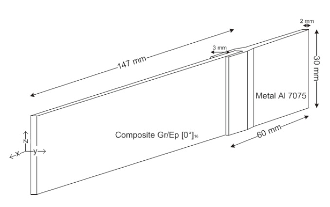
Fig. 1 shows the dimensions and the shape of the whole specimen chosen in this study, respecting constraints of the vacuum chamber used in this study. Concerning the shape, it was decided to design an oblong specimen to focus the behaviour along one axis, and to facilitate the installation of the specimen on the support of the vacuum chamber. The z-direction (gravity direction) dimension was imposed on 30 mm to have enough stiffness along this direction to avoid eventual deformations caused by the gravity field.
The composite part used in this study was [0˚]16 Gr/Ep, unidirectional along the longitudinal axis, along which its CTE was ?0.81 × 10⁻⁶ K-1. Al 7075 was employed as the metal part, and its CTE value was 23.6 × 10⁻⁶ K-1. CTE values defined in (1) were measured following the method of Kim
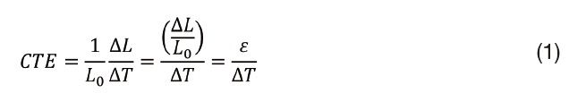
where
The metal part and the composite part were bonded together by the double lap layer bonding method, using epoxy glue. This choice was made to enable enough stiffness to bear stress due to the difference of temperature and CTEs of metal and composite parts, and to thermally isolate the materials as much as possible. The thickness of both layers of epoxy glue was 0.5 mm. This was chosen after a finite element analysis on the specimen.
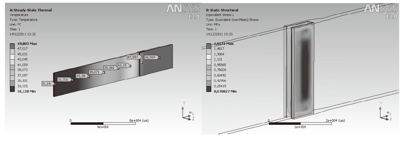
A series of finite element analyses were conducted to predict the temperature distributions, the degree of dimensional controllability, and to verify the structural integrity. In the FE analyses, the end of the metal part was fixed. Fig. 2 shows the steady-state temperature distribution and the corresponding stress distribution for a 50 ℃ temperature on the heater surface of the metal part was imposed, with an environmental temperature of 21 ℃ . Within 1 hour, the composite part reached the temperature of 31 ℃ . The results of the FE analysis in Fig. 2 also show that the maximum Von Mises stress of the epoxy glue is 1.9 MPa, far below the yield compressive strength of 36 MPa.
Interferometers are able to measure displacements without contacting the specimens controlling the environmental and geometrical error sources [13]. The DMI system is composed of a dual-mode laser head that generates HeNe laser light at a 633 nm wavelength at 3.4 and 4.0 MHz, with highly stable interferometers, reflectors, fiber optic pickups and supporting electronics. The laser consists of two beams orthogonally polarized. Two beams travel along the reference path within the interferometer and the measurement path. The length difference between the two paths induces the phase difference Δφ as shown in the following:
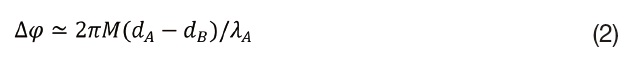
where
The displacement of the target (
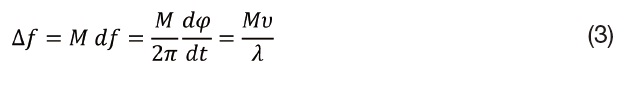
where
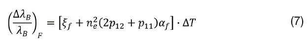
The FBG sensor is a type of fiber optic sensor, its use in space structures is being actively studied. The working principle of the FBG is based on a periodic change of the refractive index in the optical fiber. Each FBG reflects a specific wavelength (Bragg wavelength λB). The optical fiber used for the FBG sensor has its own CTE α
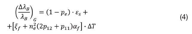
where the term pe is the photo-elastic constant of the optical fiber. p11 and p12 are the components of the strainoptic tensor, and ne is the effective refractive index of the Bragg grating.
The specimen strain
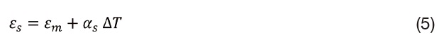
where
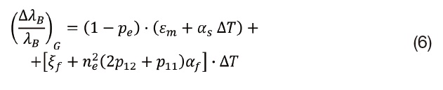
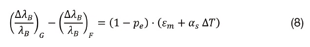
For the free FBG sensor (floating on the specimen), no specimen strain
The compensation for the temperature effect on the FBG sensor is achieved by subtracting the two relations above:
If there are no external loads, the mechanical strain
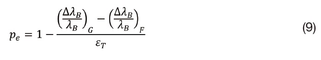
where
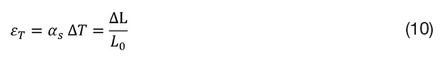
This depends exclusively on the temperature behaviour of the specimen because no mechanical stress is imposed. The value of
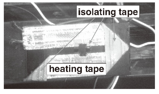
Concerning the heating tape, the resistance per length is 28 Ω/ft , and the maximum allowable power per length is 70 W/ft. It was attached on the metal part surface in one row, on both faces. The heating tape contained 4 resistive wires, embedded in 11-mm-width tape, heating the surface quasiisotropically. Fig. 3 explains the connection configuration of the heating tape. The parts, where the tape deflects from up to down, were covered with isolating tape. The little square in the centre was cut out in order to facilitate attaching the thermistor.
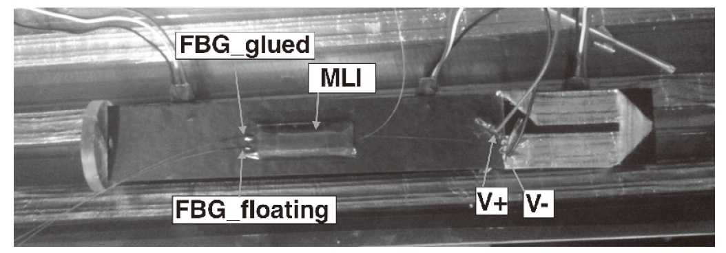
FBG sensor arrays can be easily prepared by connecting several Bragg gratings written at different wavelengths in a line along the length of a single fiber and addressing each sensor individually using wavelength division multiplexing (WDM) technology. In this case, an array of two Bragg gratings was created. As Fig. 4 shows, the first Bragg grating (
Multi-Layer Isolator (MLI). The orientation of the attached FBG should be along the longitudinal axis of the composite material.
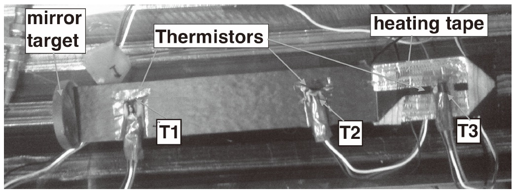
The thermistors are TO-92 Plastic Package from the LM35 series by the National Semiconductor. It does not require any external calibration or trimming to provide typical accuracies of ± 0.25 ℃ at room temperature and ± 0.75 ℃ over a full -55 ~ 150 ℃ temperature range. They were attached on specified points: the first one at 20 mm from the end of the composite part, the second one at 30 mm from the metal part and the third one in the center of the metal part, as depicted in Fig. 5. These thermistors are called T1, T2 and T3, respectively. T3 was isolated from the heating tape with a layer of isolating tape. Between the thermistors and the surface of the specimen, a layer of thermal conductive foam was used.
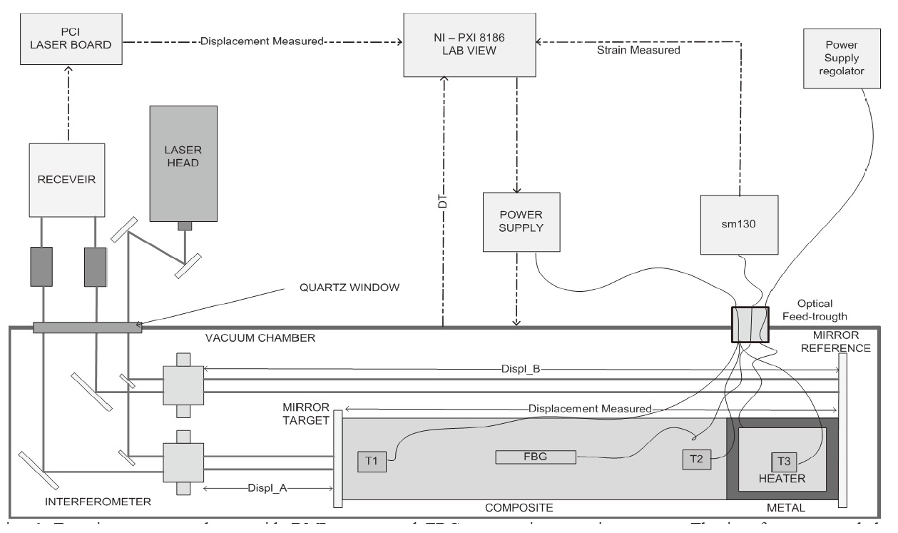
The DMI system consists of a laser head (Agilent 5517D), two plane mirror interferometers (Agilent 10706B highstability plane mirror interferometer), a specimen base with a reference mirror, a receiver (Agilent E1708A remote dynamic receiver) and a PCI laser board (Agilent N1231B).
The entire experimental setup was maintained inside of a vacuum chamber simulating the space environment in terms of pressure (on the order of 10-3 torr) and variations of temperature (± 10 ℃ in about 2 hours). Since the specimen was laid on the specimen base, the base was supported by a roller to let the specimen float with minimal friction.
Fused silica was selected as the material for the specimen base, specimen roller and reference mirror because of its very small CTE (on the order of 10?7 ℃?1). One end of the specimen was attached to the reference mirror to compensate for the specimen base’s expansion. The heating tape was connected through the optical feed-through to the power supply regulator.
The temperature of the metal part was detected with thermistor T3, and the temperature of the composite part was detected by an average of T1 and T2. All data from the DMI system, FBG sensors and thermistors were collected using a LabVIEW computer (NI PXI 8186). Fig. 6 shows the overall experimental setup scheme. The interferometers and the specimen base were placed inside the vacuum chamber. The laser head and receiver were located outside the chamber. The quartz window was installed on the vacuum chamber to let the laser light pass through. A heat tunnel, which surrounded the specimen and specimen base, was coated in black to easily transfer heat through radiation.
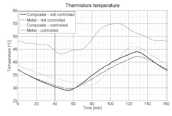
In order to facilitate the lab-scale dimensional controls, the experiment was performed in always-positive heat power delivery mode. The metal part was heated by the heating tape; and the cooling control of both parts was performed by radiation. Therefore, the temperature of the metal part was set to be higher than the ambient temperatures. The gap shall be enough to keep the temperature of the metal part higher than the composite temperature during the entire experiment, allowing the heat power of the system transferring outward by radiation during the cooling phase. Fig. 7 shows the typical temperature time course of the specimen. The vacuum chamber temperature range was set to 30~46 ℃. The initial temperature of the vacuum chamber and composite part was set at 38 ℃, and the initial temperature of the metal part was set at 47 ℃. As shown in Fig. 7 , the temperature of the metal part was set to 9 ℃ higher than ambient temperature to increase the controllability of the displacement by adjusting the voltage of the heaters during the control. The voltage range used to control the
displacement of the metal part was 0~6 V. The temperature of the composite part was the control input of the heating system. The control input was the displacement measured by the DMI system shown in Fig. 6, defined as the variation of the initial elongation of the whole specimen and the elongation during the experiment. The control output was the voltage, manipulated by the power supply in steps of 0.05 V. Control time sampling was at 1 sample per 1 minute. The minimum variation of voltage between two subsequent values was 0.1 V.
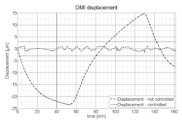
Fig. 8 clearly shows that the deformation measured by the DMI system was maintained within the tolerance of ±1 μm , which satisfies the goal of dimensional stability tolerance of ±3 μm .
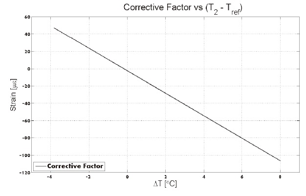
Because the bonding was not thermally isolated between both parts, a temperature gradient existed along the longitudinal direction of the specimen as shown on the left side of Fig. 2. Thus, the direct integration of strain measured by FBG was not the whole displacement of the specimen which could be measured by the DMI system. Therefore, a corrective factor with respect to the temperature difference between the composite part
where A=?1.3 × 10?5 K?1 and B=?2.5 × 10?6 are the constants of the approximating function.
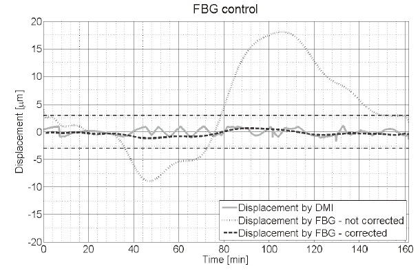
This function shall be applied to the strains by the FBG sensor. Fig. 9 shows the behaviour of the corrective factor. Fig. 10 shows that the controlled displacement based on the FBG sensors with the corrective factor remained within the tolerance of ±1 μm . Without corrective factor, the small displacement was hardly measured by using only FBG sensors. Thus, the proper corrective factor should be applied to the FBG sensors in order to use the strain data from FBG sensors as the control input.
An active dimension compensation concept for a composite structure using an additional controllable metal part was demonstrated.
From the FEM analysis, proper specimen configuration was designed. The dimensional changes of the specimen were engaged in a vacuum chamber in order to simulate space conditions, and these dimensional changes were
compensated by proper control of the temperature of the metal part. From the test, it has been shown that dimensional stability of ±1 μm was successfully achieved. In addition, the corrective factor calculated from the temperature data showed the possibility of using the FBGs as a monitoring sensor for dimensional stability.