Numerical simulations of 3D aircraft configurations are performed in order to understand the effects of turbulence models on the prediction of aircraft's aerodynamic characteristics. An in-house CFD code that solves 3D RANS equations and two-equation turbulence model equations are used. The code applies Roe’s approximated Riemann solver and an AF-ADI scheme. Van Leer’s MUSCL extrapolation with van Albada’s limiter is also adopted. Various versions of Menter’s k-ω SST turbulence models as well as Coakley’s q-ω model are incorporated into the CFD code. Menter’s k-ω SST models include the standard model, the 2003 model, the model incorporating the vorticity source term, and the model containing controlled decay. Turbulent flows over a wing are simulated in order to validate the turbulence models contained in the CFD code. The results from these simulations are then compared with computational results from the 3rd AIAA CFD Drag Prediction Workshop. Numerical simulations of the DLR-F6 wing-body and wing-body-nacelle-pylon configurations are conducted and compared with computational results of the 2nd AIAA CFD Drag Prediction Workshop. Aerodynamic characteristics as well as flow features are scrutinized with respect to the turbulence models. The results obtained from each simulation incorporating Menter’s k-ω SST turbulence model variations are compared with one another.
b Wing Span
CL Lift coefficient
CD, CDf, CDp Total drag, skin friction drag, pressure drag
Cω1, Cω2, Cω3, Cq1 Model constants of q-ω turbulence model
k Turbulent kinetic energy
p Pressure
q Turbulent velocity scale
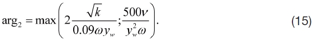
yw Nearest distance to the wall

Span-wise distance measured from fuselage centerline
α, β, β* Model constants of k-ω SST turbulence model
μm Molecular viscosity
μt Turbulent viscosity
σS1, σS2 Model constants of the turbulence models
ω Turbulent dissipation rate
Ω Absolute value of vorticity
Computational Fluid Dynamics (CFD) is a major research tool for aircraft design and analysis. However, predicting aerodynamic characteristics is difficult because of aircraft's complex flow features and configurations. Turbulent flow comprises the majority of the flows around an aircraft; it is often accompanied by large separations, wall shear layers, and shocks. Resolving the entire range of turbulent length scales is necessary for accurately analyzing the flow. However, the high computational expenses connected to Direct Numerical Simulation (DNS) forces us to use some sort of turbulence modeling in the simulation of complex flows around aircraft. The Reynolds Averaged Navier-Stokes (RANS) equations are more effective than Large Eddy Simulation (LES) for turbulence modeling. However, the choice of turbulence models strongly influences the RANS solutions. Thus, selecting an appropriate turbulence model requires special care and attention.
The aerodynamic characteristics of an aircraft were researched at the AIAA CFD Drag Prediction Workshops (DPW). At the 2nd AIAA CFD DPW (DPW-2) [1], the DLR-F6 wing-body (WB) model and wing-body-nacellepylon (WBNP) model were selected for drag prediction. Experimental data and results from the participants in DPW- 2 are presented on the website [1] as well as at the 42nd AIAA Reno conference. At the 3rd AIAA CFD DPW (DPW-3) [2], the DLR-F6 wing-body with FX2B fairing transport model and wing-only models (DPW-W1 and W2) were selected to predict aircraft forces and moments. The FX2B fairing reduced separation at the wing-body juncture. DPW-W1 and W2 are transonic wing models suitable for validating the code. Experimental data and numerical results are summarized on the website [2].
The purpose of this paper is to evaluate the aerodynamic characteristics of 3D aircraft configurations according to the various turbulence models. This is undertaken using an inhouse CFD code, which is validated through comparison between the numerical results and other computational results for the DPW-W1 model. Numerical simulations of the DLR-F6 WB model and the WBNP model are then performed using various turbulence models including the
In this paper, the governing equations and numerical schemes for the mean flow are first presented. Next, various turbulence models are briefly discussed. The simulation results of the DPW-W1 model are presented to show the validity of the code. The aerodynamic characteristics of the DLR-F6 WB and WBNP models are presented and compared with other research results.
2.1 Governing Equations and Numerical schemes
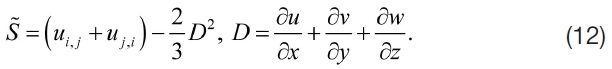
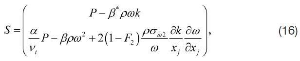
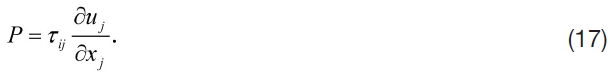
Three-dimensional RANS equations and the two-equation turbulence model equations are chosen as the governing equations for the simulation of the turbulent flow around an aircraft. The equations are
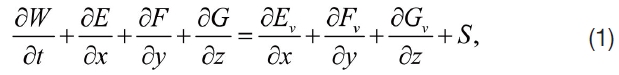
where


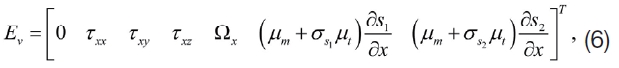
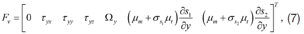
where
The governing equations are solved using a cell centered Finite Volume Method (FVM). Roe’s approximated Riemann solver [3] is used for computing the inviscid flux; the central difference method is employed for the viscous flux. Van Leer’s MUSCL extrapolation [4] with a limiter is used to obtain second-order accuracy while maintaining the Total Variation Diminishing (TVD) property. An Approximate Factorization-Alternative Direction Implicit (AF-ADI) scheme [5] is used for the steady-state solution.
Coakley’s
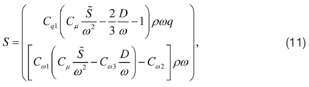
2.2.1 Coakley’s q-ω model
The turbulent velocity scale,
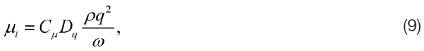
where
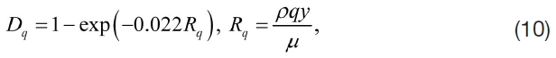
where
2.2.2 Menter’s k-ω SST Model (SST) and Its Various Versions
Menter’s
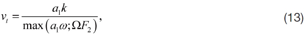
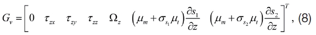
The source term vector is defined as
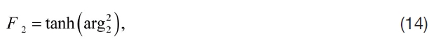
The other model constants are determined with blending function
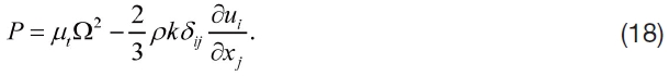
2.2.3 SST Model with the Vorticity Source Term (SST-V)
The vorticity magnitude is more easily computed in comparison to the exact source term. The vorticity magnitude is generally very close to the exact source term in simple boundary layer flows. In this model, the term
2.2.4 SST Model from 2003 (SST-2003)
The SST-2003 model redefines the eddy viscosity term. Eddy viscosity is computed using the strain invariant rather than the vorticity magnitude.
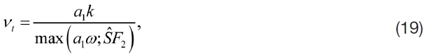
where
While the production limiter is used for the
2.2.5 SST Model with Controlled Decay (SST-sust)
For external aeronautical flows, the SST model with controlled decay (SST-sust) prevents the non-physical decay of the turbulence variables in the free-stream. Sustaining terms are added to the source term in the turbulence equations; the changed source term vector is therefore redefined as follows:
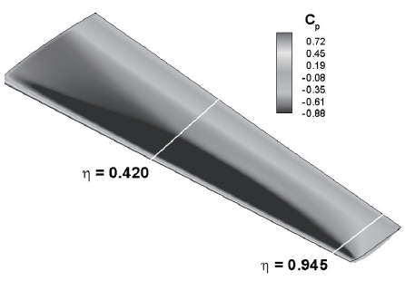
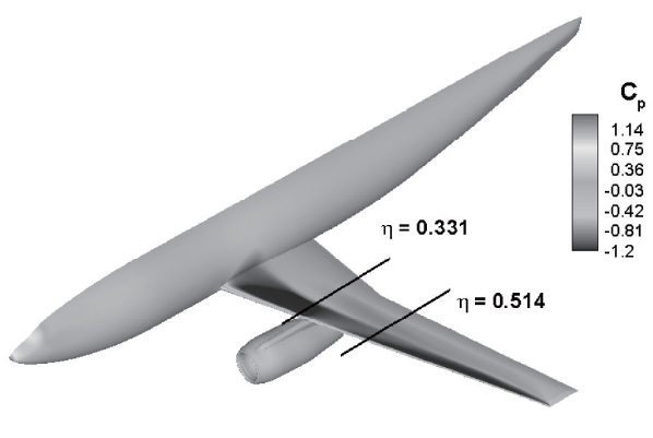
Numerical simulations of the DPW-W1 configuration are conducted to validate the CFD code. The results are then compared with computational results by Tinoco [2]. The Mach number of the flow is 0.76 and the Reynolds number is 5.0× 10⁶ based on a Mean Aerodynamic Chord (MAC) length of 197.556 mm. The angle of attack (AOA) is 0.5 degree. The grid used in Tinoco’s research is employed in these simulations. The

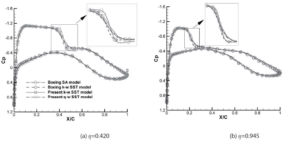
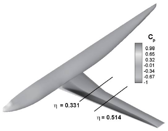
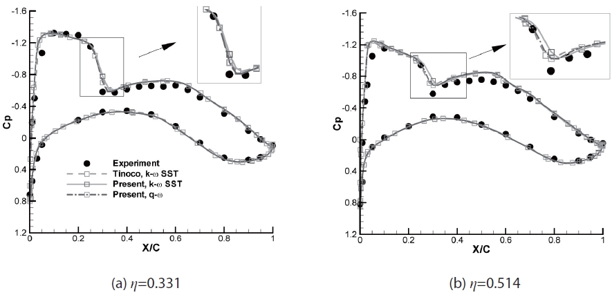
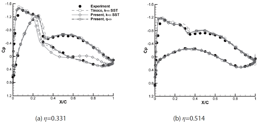
used for the comparisons of pressure distributions are presented in Fig. 1. Pressure coefficient distributions around the upper surface are also shown. Comparisons between the pressure distributions
in the two positions are shown in Fig. 2; the pressure distributions correlate well with Tinoco’s results except close to the shock locations, where there are slight differences in pressure. However, determining which results are more accurate is difficult without experimental data.
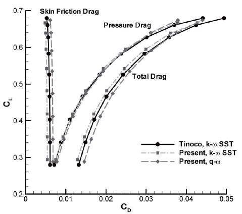
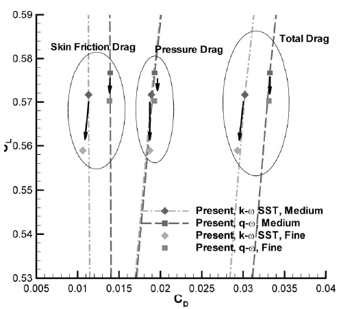
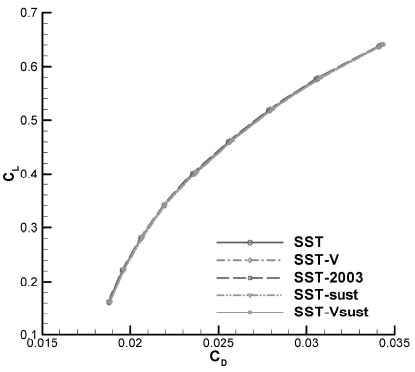
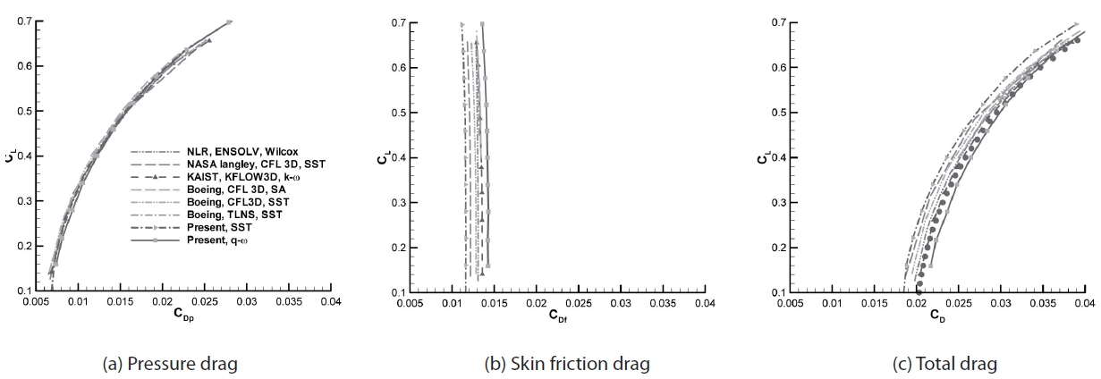
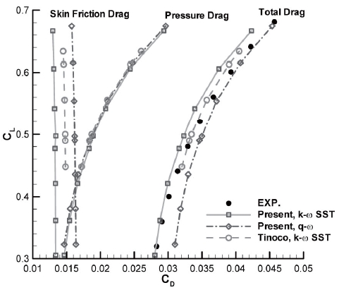
Drag polars computed by the current code are compared with Tinoco’s results in Fig. 3; there is good agreement in the pressure drags, while the calculated skin friction drags differ. Thus, the difference between the total drag coefficients is due to discrepancies in the values of skin friction drag. The pressure differences near the shock locations have little effect on the aerodynamic coefficients. Relative to Tinoco’s results, the total drag in the
Changes in aerodynamic characteristics with respect to turbulence models are explored through simulations of the
flows around the DLR-F6 WB configuration. The compared turbulence models are the
The DLR-F6 WB configuration and the pressure coefficient distribution along the surface are presented in Fig. 6. The span locations of the pressure distributions are also displayed. The figure shows that the shock is clearly established on the upper surface of the wing. The angle of attack and the drag coefficients of the present results and experimental work at the design cruise condition are listed in Tab. 1. A centerline and scatter limits are also presented. The median (Med.) and the scatter limits are computed by statistical methods and used for comparison of the code-tocode scatter [11]. The limits (upper limit : Up., lower limit : Lo.) provide a reasonable estimate of the population mean and the standard deviation of the core solutions. The table shows that the present results fall within the limits. The
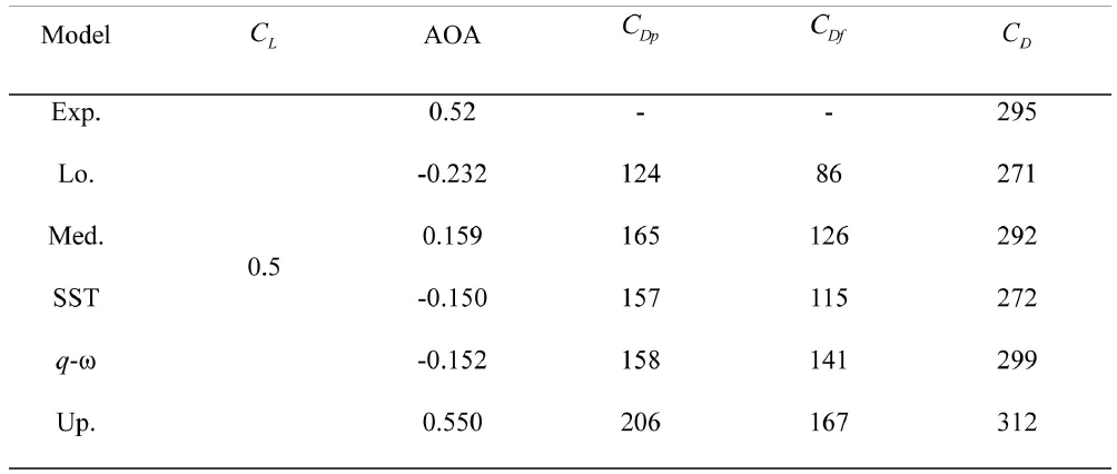
Angles of attack and values of drag at the design cruise condition (AOA : deg, Drag: counts)
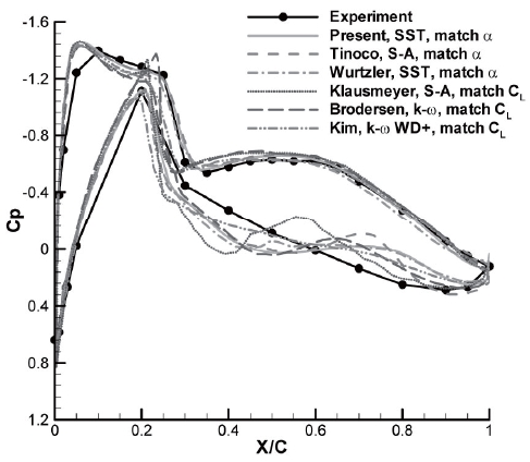
Comparisons of the pressure distributions at the two span positions are presented in the Fig. 7. At
In Fig. 8, the drag polars are compared with other numerical results and with experimental data. The drag polars of the pressure drag exhibit little differences between the sets of results, but the skin friction drag shows a larger difference, demonstrating that the turbulence model significantly influences predictions of aerodynamic characteristics. The lowest calculated total drag value is from the
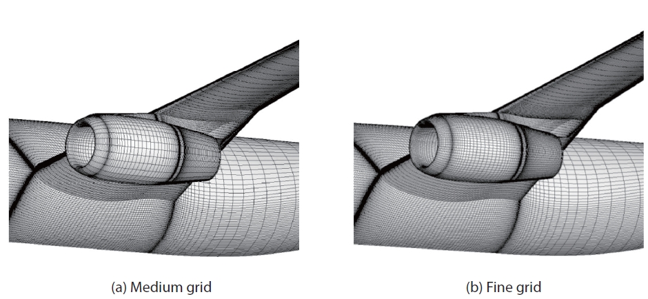
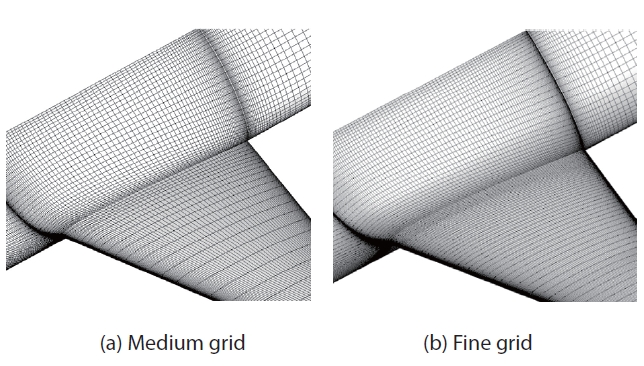
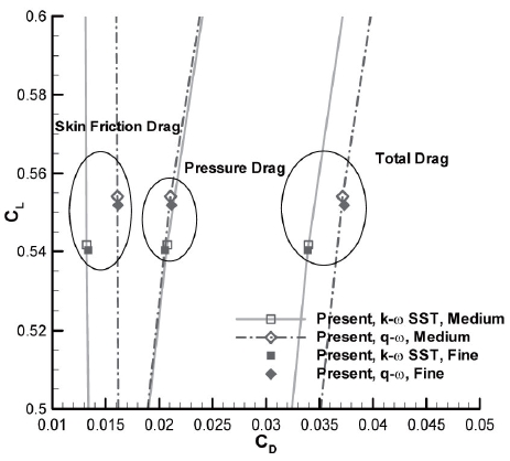
Simulations of the WBNP configuration are conducted under the same flow conditions as the WB configuration using Tinoco's medium (6.2 million grid points) and fine (8.7 million grid points) grid systems. Magnified views of the grids on the surface near nacelle and pylon are shown in Fig. 10. The changes of drag and lift using the two grids are shown in Fig. 11. The same movement in the drag polars is found with the fine grid system as in the WB configuration. The configuration of the WBNP and the pressure distributions around the wing are depicted in Fig. 12. The two
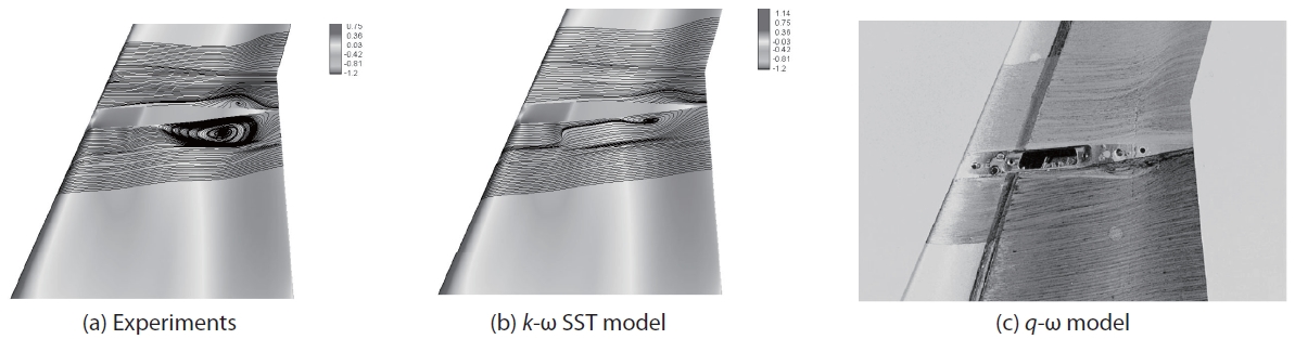
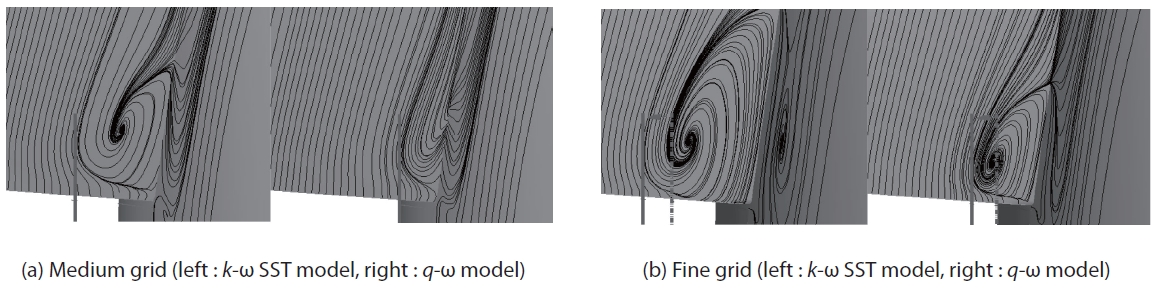
The stream-traces on the upper surface of the wing near the wing-body junction are shown in Fig. 14. The flow region with the
model. These results suggest that simulation under a certain combination of grid density and turbulence model results in excessive flow separation on the wing surface near the pylon.
The drag polars are compared to Tinoco’s results and experimental data in Fig. 17. As in DPW-W1 and WB, significant differences are not observed between the pressure drags, but the skin friction drag coefficients differ from Tinoco’s results. Thus, the turbulence model would be the greatest influence on the drag coefficient in the all simulations. The skin friction drags are underestimated by the
drag coefficients obtained from the
Simulations of aircraft configurations were performed using various turbulence models to understand an aircraft’s aerodynamic characteristics. The
of the WB configuration, the